Как проще всего запустить rstudio в операционной системе windows

Перевод инструкции с DataCamp

Инструкция для начинающих, которая спасёт вас от головной боли и сэкономит время тем, кто решил установить R самостоятельно.

R — один из основных языков используемых сегодня в науке о данных. Поэтому любой, кому интересна эта сфера, может захотеть узнать, как начать пользоваться R вне зависимости от операционной системы, установленной на компьютере. Это руководство поможет установить R на Windows 10, Mac OS X и Ubuntu Linux.

Кроме того, в руководстве рассматриваются установка RStudio, мощной IDE (Integrated Development Environment, интегрированная среда разработки), упрощающей программирование на R, и установка пакетов для R, таких как dplyr или ggplot2.

С установкой R на Windows 10 нет никаких сложностей. Самый простой способ — установить его через CRAN (расшифровывается как The Comprehensive R Archive Network). Перейдите на страницу загрузок CRAN и проследуйте по ссылкам из анимации ниже:

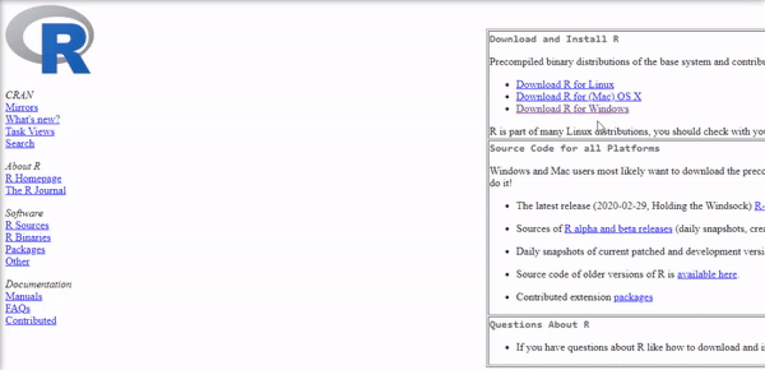
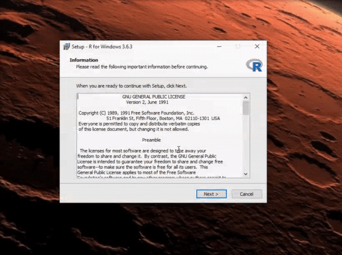
Как только загрузка будет завершена, вы найдёте у себя файл под названием «R-3.6.3-win.exe» (либо похожим — в зависимости от номера версии R, которую вы скачаете). Ссылки в анимации выше помогут вам скачать самую актуальную версию. Всё, что осталось сделать для завершения установки R, это запустить загруженный exe-файл. По большей части, вам нужно просто соглашаться с опциями по умолчанию, так что просто нажимаете кнопку «Next» до завершения установки, как показано в следующей анимации. Обратите внимание, что на одном из экранов можно добавить иконки для вызова R через панель быстрого доступа и с рабочего стола (в анимации выбрана опция «Не добавлять».

Установка RStudio

Как только установлен R, вы можете установить RStudio, намного более мощный редактор для скриптов R. Среди прочего, RStudio включает в себя консоль, поддерживающую непосредственное исполнение кода, а также инструменты для построения графиков и отслеживания переменных в вашем рабочем пространстве. Процесс установки также прост. Просто перейдите на сайт RStudio и повторяйте за анимацией:

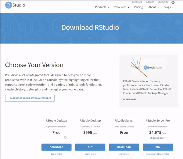
Когда загрузка закончится, вы получите файл «RStudio-1.2.5033.exe», или с похожим названием — снова, в зависимости от версии. Запустите его, согласитесь с предлагаемыми по умолчанию настройками, нажимая кнопку «Next» и дождитесь окончания установки — как и в прошлый раз. Помните, что перед установкой RStudio необходимо установить R!

Установка пакетов в R

У вас уже установлены R и отличная IDE — можно начинать программировать. Однако, базовая версия R очень ограничена в возможностях, поэтому сообщество пользуется дополнительными пакетами, расширяющими функционал языка, такими как dplyr (расширяет возможности обработки данных) или ggplot2 (предоставляет улучшенные инструменты для визуализации). Есть два способа установки пакетов для R через RStudio. Первый — выполнить следующий код в консоли:

install.packages(c("dplyr","ggplot2"))

Второй способ показан в анимации ниже. Это лёгкий в использовании графический интерфейс, встроенный в RStudio, благодаря которому вы сможете найти и загрузить любой пакет для R, доступный в CRAN.

Установка R на Mac OS X

Процесс установки R на Mac OS почти не отличается от установки на Windows. Снова, самый простой способ — загрузить установщик со страницы загрузок CRAN:

Следующий шаг — запуск файла «R-3.6.2.pkg» (или более новой версии). Также, как и в Windows, можно оставить все опции по умолчанию.

Установка RStudio и пакетов R

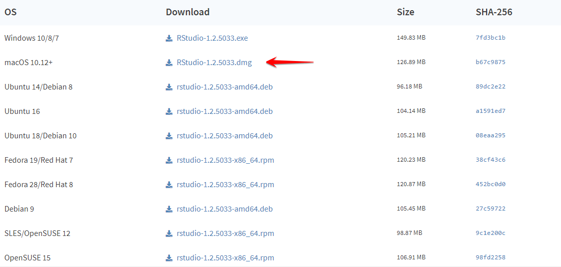
В обоих случаях отличий от установки в Windows нет. Для загрузки RStudio перейдите на страницу загрузки и скачайте файл с расширением .dmg для Mac OS (как на картинке ниже). Оставляйте выборы по умолчанию.

Откройте RStudio. Установка пакетов проходит также, как в Windows. Можно ввести в консоль команду

install.packages(c("dplyr","ggplot2"))

или воспользоваться графическим интерфейсом, показанным в части «Установка пакетов в R» этого руководства.

Установка R в Ubuntu 19.04/18.04/16.04

Установка R в Ubuntu может быть несколько более сложной для тех, кто не привык работать в командной строке (консоли). Тем не менее, это практически также просто, как и в случаях с Windows или Mac OS. Прежде чем начать, убедитесь, что у вас есть права уровня root, позволяющие пользоваться sudo.

Как обычно, перед установкой R, давайте обновим список системных пактов, и обновим установленные пакеты, воспользовавшись двумя следующими командами:

sudo apt update

sudo apt -y upgrade

После этого, всё, что необходимо сделать для установки R — выполнить в консоли следующую команду:

sudo apt -y install r-base

Установка RStudio и пакетов R

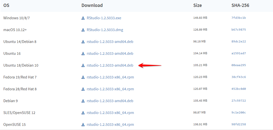
Когда базовый R установлен, вы можете установить RStudio. Переходим на страницу загрузок, выбираем .deb файл для нашей версии Ubuntu, как на картинке ниже:

Когда вы скачали .deb файл, всё, что осталось сделать, это перейти в папку с загрузками, воспользовавшись командой

cd Downloads

и запустить оттуда процесс установки командой

sudo dpkg -i rstudio-1.2.5033-amd64.deb

Вы можете столкнуться с некоторыми проблемами с зависимостями, которые не дадут вам установить RStudio с первой попытки, но исправить эти проблемы очень легко. Выполните следующую команду и попробуйте снова:

sudo apt -f install

Когда установка закончится, иконка RStudio появится в списке приложений в Ubuntu, но вы также сможете запустить программу набрав rstudio в консоли.

В запущенной RStudio установка пакетов происходит ровно также, как в Windows или Mac OS. Либо введите

install.packages(c("dplyr","ggplot2"))

либо воспользуйтесь графическим интерфейсом, как показано в части «Установка пакетов в R» этого руководства.

Заключение

Я надеюсь, что это руководство поможет тем из вас, кто желает погрузиться в мир программирования на R вне зависимости от операционной системы, которой вы пользуетесь. Если вам интересно узнать о возможностях языка, воспользуйтесь курсом Введение в R от DataCamp, который познакомит вас с основами. Продолжайте учиться, нет предела совершенству!

[This article was first published on R tutorial – Dataquest, and kindly contributed to R-bloggers]. (You can report issue about the content on this page here)

---

Want to share your content on R-bloggers? click here if you have a blog, or here if you don’t.

In this tutorial we’ll learn how to begin programming with R using RStudio. We’ll install R, and RStudio RStudio, an extremely popular development environment for R. We’ll learn the key RStudio features in order to start programming in R on our own.

If you already know how to use RStudio and want to learn some tips, tricks, and shortcuts, check out this Dataquest blog post.

Table of Contents

• 1. Install R
• 2. Install RStudio
• 3. First Look at RStudio
• 4. The Console
• 5. The Global Environment
• 6. Install the tidyverse Packages
• 7. Load the tidyverse Packages into Memory
• 8. Identify Loaded Packages
• 9. Get Help on a Package
• 10. Get Help on a Function
• 11. RStudio Projects
• 12. Save Your “Real” Work. Delete the Rest.
• 13. R Scripts
• 14. Run Code
• 15. Access Built-in Datasets
• 16. Style
• 17. Reproducible Reports with R Markdown
• 18. Use RStudio Cloud
• 19. Get Your Hands Dirty!
• Additional Resources
• Bonus: Cheatsheets

RStudio is an open-source tool for programming in R. RStudio is a flexible tool that helps you create readable analyses, and keeps your code, images, comments, and plots together in one place. It’s worth knowing about the capabilities of RStudio for data analysis and programming in R.

Using RStudio for data analysis and programming in R provides many advantages. Here are a few examples of what RStudio provides:

• An intuitive interface that lets us keep track of saved objects, scripts, and figures
• A text editor with features like color-coded syntax that helps us write clean scripts
• Auto complete features save time
• Tools for creating documents containing a project’s code, notes, and visuals
• Dedicated Project folders to keep everything in one place

RStudio can also be used to program in other languages including SQL, Python, and Bash, to name a few.

But before we can install RStudio, we’ll need to have a recent version of R installed on our computer.

1. Install R

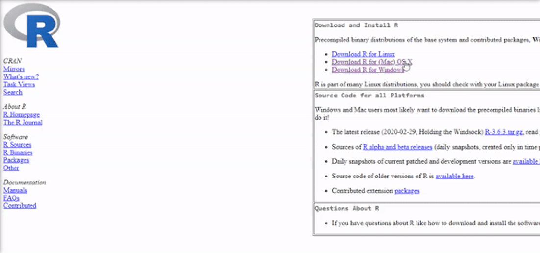
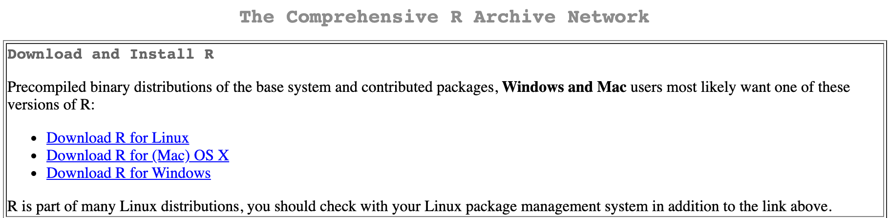
R is available to download from the official R website. Look for this section of the web page:

The version of R to download depends on our operating system. Below, we include installation instructions for Mac OS X, Windows, and Linux (Ubuntu).

MAC OS X

• Select the Download R for (Mac) OSX option.
• Look for the most up-to-date version of R (new versions are released frequently and appear toward the top of the page) and click the .pkg file to download.
• Open the .pkg file and follow the standard instructions for installing applications on MAC OS X.
• Drag and drop the R application into the Applications folder.

Windows

• Select the Download R for Windows option.
• Select base, since this is our first installation of R on our computer.
• Follow the standard instructions for installing programs for Windows. If we are asked to select Customize Startup or Accept Default Startup Options, choose the default options.

Linux/Ubuntu

• Select the Download R for Linux option.
• Select the Ubuntu option.
• Alternatively, select the Linux package management system relevant to you if you are not using Ubuntu.

RStudio is compatible with many versions of R (R version 3.0.1 or newer as of July, 2020). Installing R separately from RStudio enables the user to select the version of R that fits their needs.

2. Install RStudio

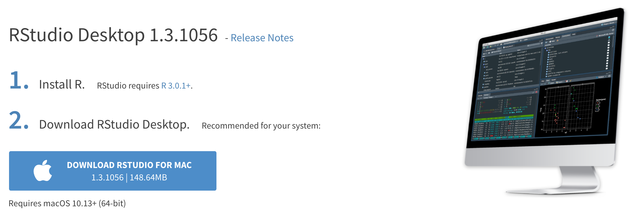
Now that R is installed, we can install RStudio. Navigate to the RStudio downloads page.

When we reach the RStudio downloads page, let’s click the “Download” button of the RStudio Desktop Open Source License Free option:

Our operating system is usually detected automatically and so we can directly download the correct version for our computer by clicking the “Download RStudio” button. If we want to download RStudio for another operating system (other than the one we are running), navigate down to the “All installers” section of the page.

3. First Look at RStudio

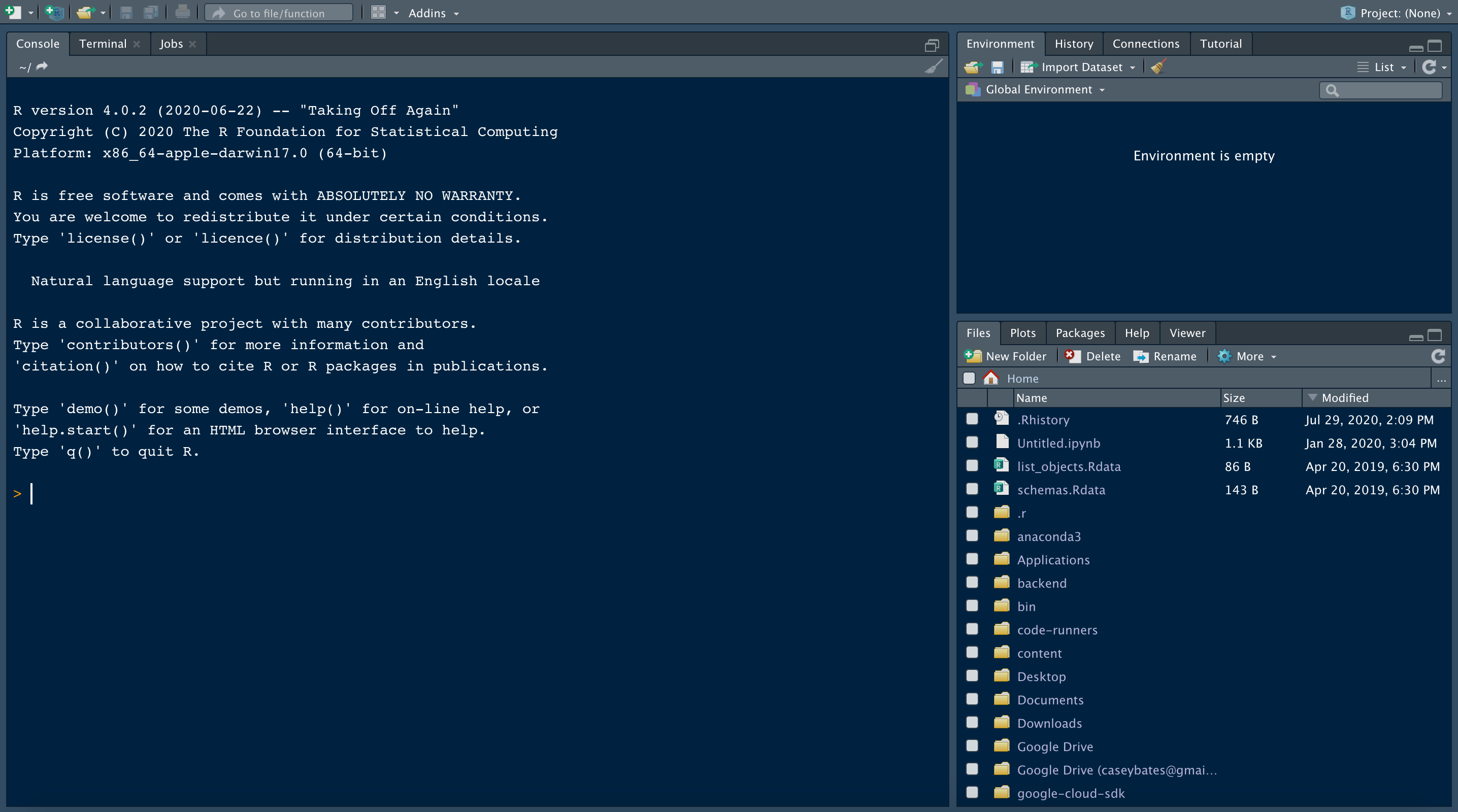
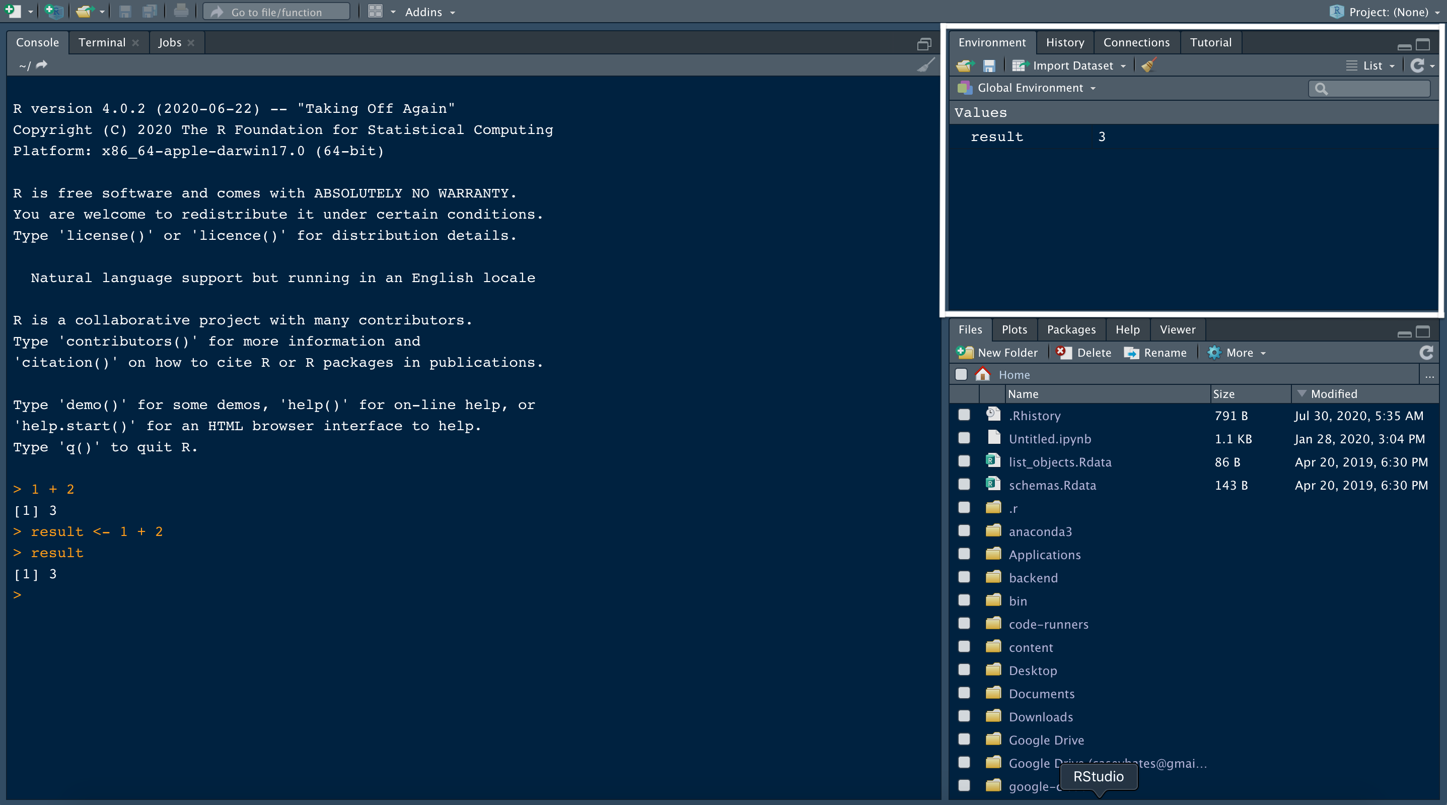
When we open RStudio for the first time, we’ll probably see a layout like this:

But the background color will be white, so don’t expect to see this blue-colored background the first time RStudio is launched. Check out this Dataquest blog to learn how to customize the appearance of RStudio.

When we open RStudio, R is launched as well. A common mistake by new users is to open R instead of RStudio. To open RStudio, search for RStudio on the desktop, and pin the RStudio icon to the preferred location (e.g. Desktop or toolbar).

4. The Console

Let’s start off by introducing some features of the Console. The Console is a tab in RStudio where we can run R code.

Notice that the window pane where the console is located contains three tabs: Console, Terminal and Jobs (this may vary depending on the version of RStudio in use). We’ll focus on the Console for now.

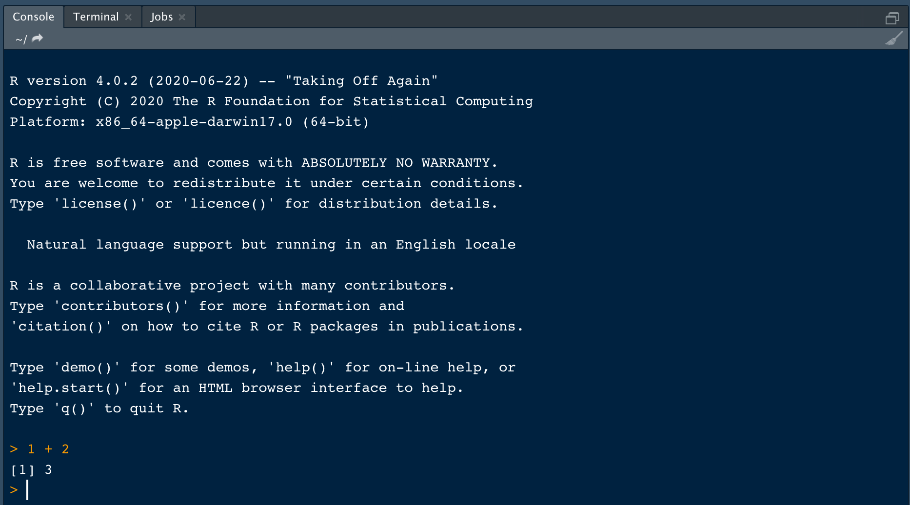
When we open RStudio, the console contains information about the version of R we’re working with. Scroll down, and try typing a few expressions like this one. Press the enter key to see the result.

1 + 2

As we can see, we can use the console to test code immediately. When we type an expression like 1 + 2, we’ll see the output below after hitting the enter key.

We can store the output of this command as a variable. Here, we’ve named our variable result:

result <- 1 + 2

The <- is called the assignment operator. This operator assigns values to variables. The command above is translated into a sentence as:

The result variable gets the value of one plus two.

One nice feature from RStudio is the keyboard shortcut for typing the assignment operator <-:

• Mac OS X: Option + -
• Windows/Linux: Alt + -

We highly recommend that you memorize this keyboard shortcut because it saves a lot of time in the long run!

When we type result into the console and hit enter, we see the stored value of 3:

> result <- 1 + 2
> result
[1] 3

When we create a variable in RStudio, it saves it as an object in the R global environment. We’ll discuss the environment and how to view objects stored in the environment in the next section.

5. The Global Environment

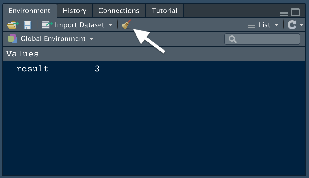
We can think of the global environment as our workspace. During a programming session in R, any variables we define, or data we import and save in a dataframe, are stored in our global environment. In RStudio, we can see the objects in our global environment in the Environment tab at the top right of the interface:

We’ll see any objects we created, such as result, under values in the Environment tab. Notice that the value, 3, stored in the variable is displayed.

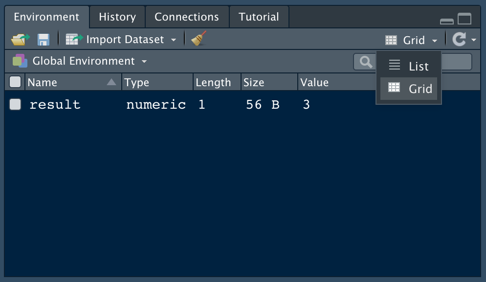
Sometimes, having too many named objects in the global environment creates confusion. Maybe we’d like to remove all or some of the objects. To remove all objects, click the broom icon at the top of the window:

To remove selected objects from the workspace, select the Grid view from the dropdown menu:

Here we can check the boxes of the objects we’d like to remove and use the broom icon to clear them from our Global Environment.

6. Install the tidyverse Packages

Much of the functionality in R comes from using packages. Packages are shareable collections of code, data, and documentation. Packages are essentially extensions, or add-ons, to the R program that we installed above.

One of the most popular collection of packages in R is known as the “tidyverse”. The tidyverse is a collection of R packages designed for working with data. The tidyverse packages share a common design philosophy, grammar, and data structures. Tidyverse packages “play well together”. The tidyverse enables you to spend less time cleaning data so that you can focus more on analyzing, visualizing, and modeling data.

Let’s learn how to install the tidyverse packages. The most common “core” tidyverse packages are:

• readr, for data import.
• ggplot2, for data visualization.
• dplyr, for data manipulation.
• tidyr, for data tidying.
• purrr, for functional programming.
• tibble, for tibbles, a modern re-imagining of dataframes.
• stringr, for string manipulation.
• forcats, for working with factors (categorical data).

To install packages in R we use the built-in install.packages() function. We could install the packages listed above one-by-one, but fortunately the creators of the tidyverse provide a way to install all these packages from a single command. Type the following command in the Console and hit the enter key.

install.packages("tidyverse")

The install.packages() command only needs to be used to download and install packages for the first time.

7. Load the tidyverse Packages into Memory

After a package is installed on a computer’s hard drive, the library() command is used to load a package into memory:

library(readr)
library(ggplot2)

Loading the package into memory with library() makes the functionality of a given package available for use in the current R session. It is common for R users to have hundreds of R packages installed on their hard drive, so it would be inefficient to load all packages at once. Instead, we specify the R packages needed for a particular project or task.

Fortunately, the core tidyverse packages can be loaded into memory with a single command. This is how the command and the output looks in the console:

library(tidyverse)## ── Attaching packages ───────────────────────────────────────────────── tidyverse 1.3.0 ──## ✓ ggplot2 3.3.2 ✓ purrr 0.3.4
## ✓ tibble 3.0.3 ✓ dplyr 1.0.0
## ✓ tidyr 1.1.0 ✓ stringr 1.4.0
## ✓ readr 1.3.1 ✓ forcats 0.5.0## ── Conflicts ──────────────────────────────────────────────────── tidyverse_conflicts() ──
## x dplyr::filter() masks stats::filter()
## x dplyr::lag() masks stats::lag()

The Attaching packages section of the output specifies the packages and their versions loaded into memory. The Conflicts section specifies any function names included in the packages that we just loaded to memory that share the same name as a function already loaded into memory. Using the example above, now if we call the filter() function, R will use the code specified for this function from the dplyr package. These conflicts are generally not a problem, but it’s worth reading the output message to be sure.

8. Identify Loaded Packages

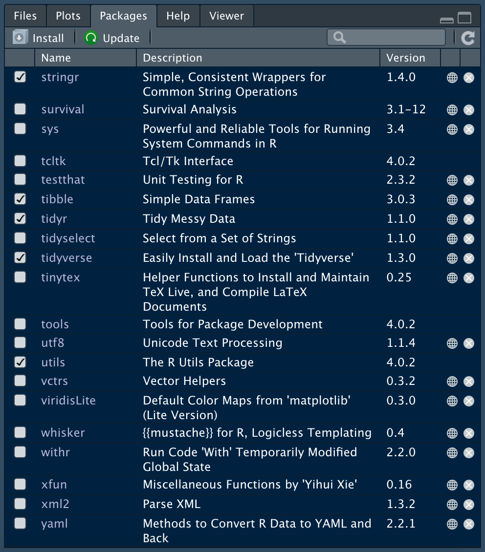
If we need to check which packages we loaded, we can refer to the Packages tab in the window at the bottom right of the console.

We can search for packages, and checking the box next to a package loads it (the code appears in the console).

Alternatively, entering this code into the console will display all packages currently loaded into memory:

(.packages())

Which returns:

[1] "forcats" "stringr" "dplyr" "purrr" "tidyr" "tibble" "tidyverse"
[8] "ggplot2" "readr" "stats" "graphics" "grDevices" "utils" "datasets" 
[15] "methods" "base"

Another useful function for returning the names of packages currently loaded into memory is search():

> search()
 [1] ".GlobalEnv" "package:forcats" "package:stringr" "package:dplyr" 
 [5] "package:purrr" "package:readr" "package:tidyr" "package:tibble" 
 [9] "package:ggplot2" "package:tidyverse" "tools:rstudio" "package:stats" 
[13] "package:graphics" "package:grDevices" "package:utils" "package:datasets" 
[17] "package:methods" "Autoloads" "package:base" 

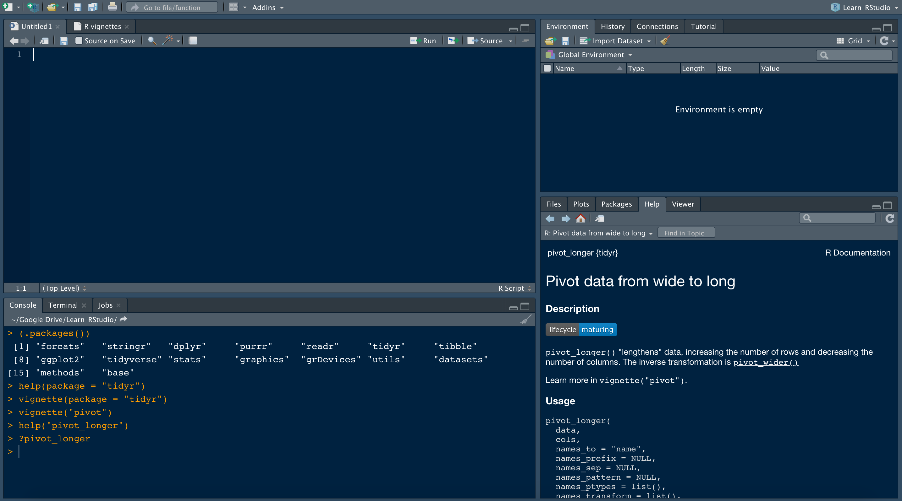
9. Get Help on a Package

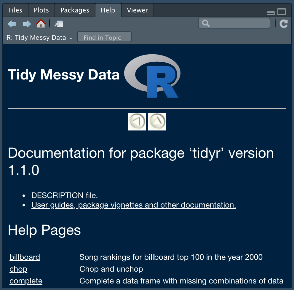
We’ve learned how to install and load packages. But what if we’d like to learn more about a package that we’ve installed? That’s easy! Clicking the package name in the Packages tab takes us to the Help tab for the selected package. Here’s what we see if we click the tidyr package:

Alternatively, we can type this command into the console and achieve the same result:

help(package = "tidyr")

The help page for a package provides quick access to documentation for each function included in a package. From the main help page for a package you can also access “vignettes” when they are available. Vignettes provide brief introductions, tutorials, or other reference information about a package, or how to use specific functions in a package.

vignette(package = "tidyr")

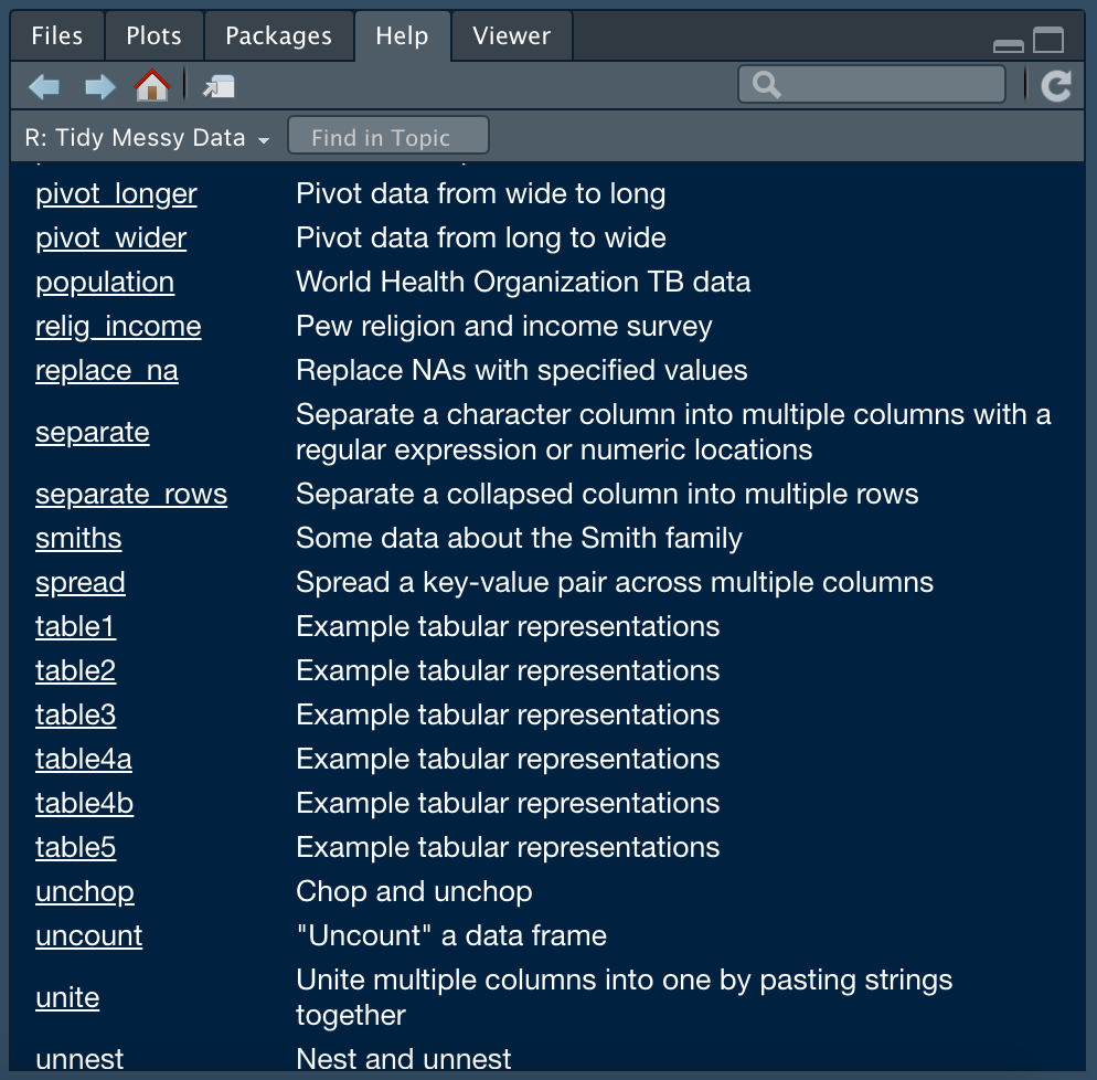
Which results in this list of available options:

Vignettes in package ‘tidyr’:nest nest (source, html)
pivot Pivoting (source, html)
programming Programming with tidyr (source, html)
rectangle rectangling (source, html)
tidy-data Tidy data (source, html)
in-packages Usage and migration (source, html)

From there, we can select a particular vignette to view:

vignette("pivot")

Now we see the Pivot vignette is displayed in the Help tab. This is one example of why RStudio is a powerful tool for programming in R. We can access function and package documentation and tutorials without leaving RStudio!

10. Get Help on a Function

As we learned in the last section, we can get help on a function by clicking the package name in Packages and then click on a function name to see the help file. Here we see the pivot_longer() function from the tidyr package is at the top of this list:

And if we click on “pivot_longer” we get this:

We can achieve the same results in the Console with any of these function calls:

help("pivot_longer")
help(pivot_longer)
?pivot_longer

Note that the specific Help tab for the pivot_longer() function (or any function we’re interested in) may not be the default result if the package that contains the function is not loaded into memory yet. In general it’s best to ensure a specific package is loaded before seeking help on a function.

11. RStudio Projects

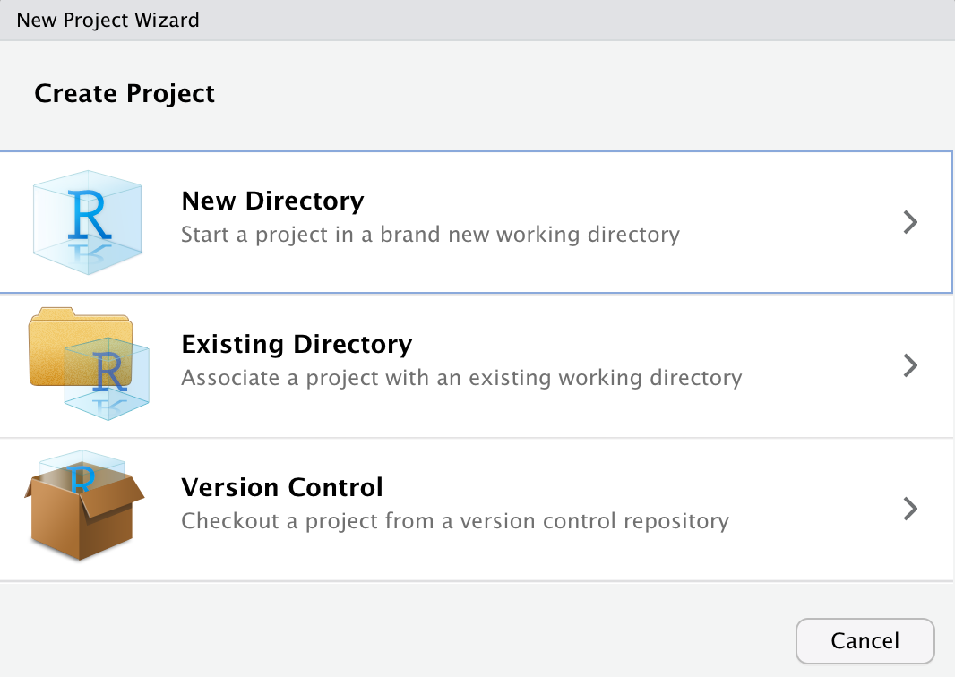
RStudio offers a powerful feature to keep you organized; Projects. It is important to stay organized when you work on multiple analyses. Projects from RStudio allow you to keep all of your important work in one place, including code scripts, plots, figures, results, and datasets.

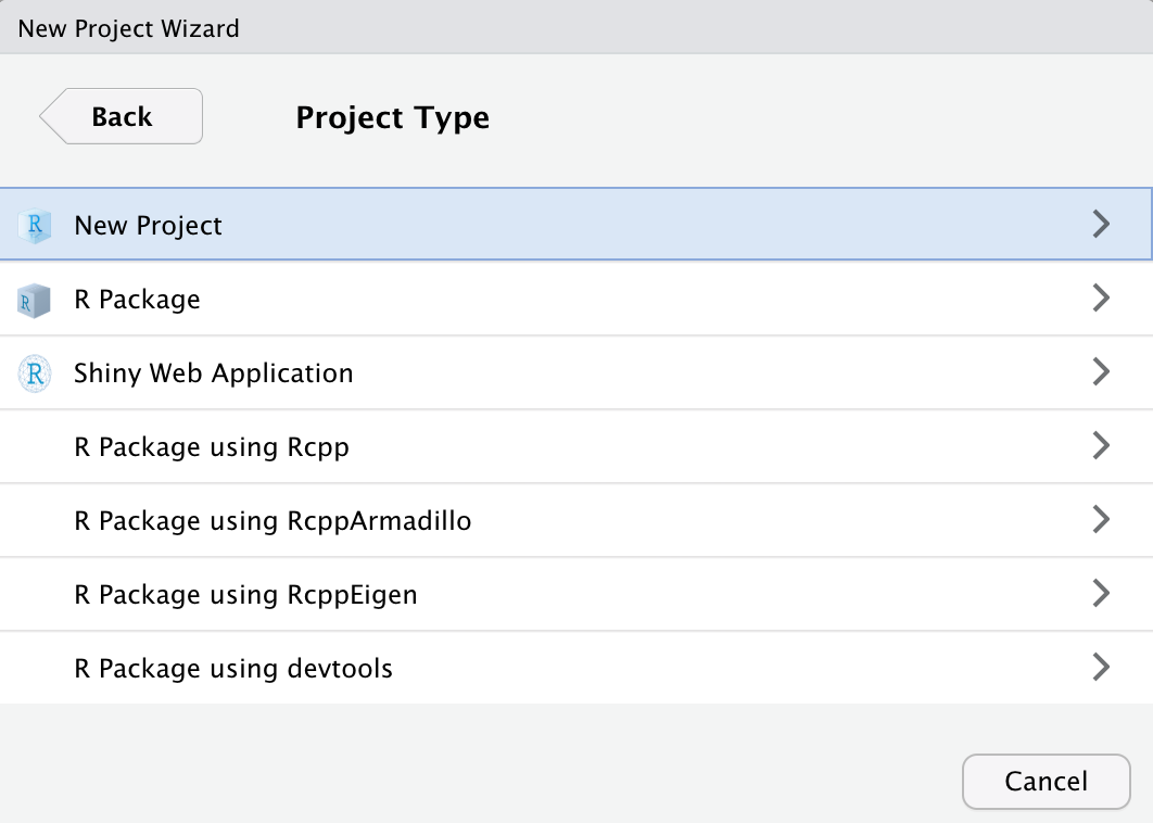
Create a new project by navigating to the File tab in RStudio and select New Project.... Then specify if you would like to create the project in a new directory, or in an existing directory. Here we select “New Directory”:

RStudio offers dedicated project types if you are working on an R package, or a Shiny Web Application. Here we select “New Project”, which creates an R project:

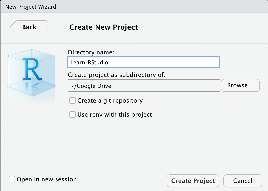
Next, we give our project a name. “Create project as a subdirectory of:” is showing where the folder will live on the computer. If we approve of the location select “Create Project”, if we do not, select “Browse” and choose the location on the computer where this project folder should live.

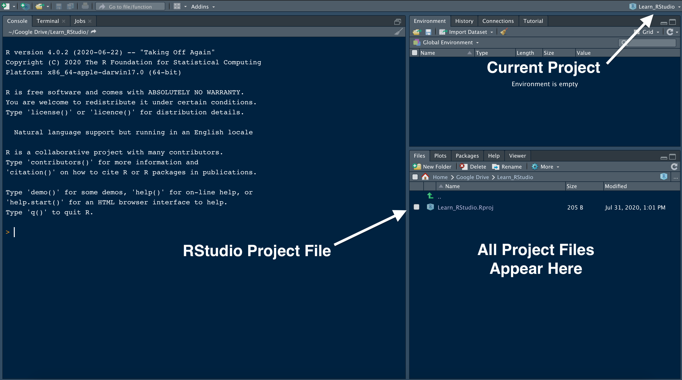
Now in RStudio we see the name of the project is indicated in the upper-right corner of the screen. We also see the .Rproj file in the Files tab. Any files we add to, or generate-within, this project will appear in the Files tab.

RStudio Projects are useful when you need to share your work with colleagues. You can send your project file (ending in .Rproj) along with all supporting files, which will make it easier for your colleagues to recreate the working environment and reproduce the results.

12. Save Your “Real” Work. Delete the Rest.

This tip comes from our 23 RStudio Tips, Tricks, and Shortcuts blog post, but it’s so important that we are sharing it here as well!

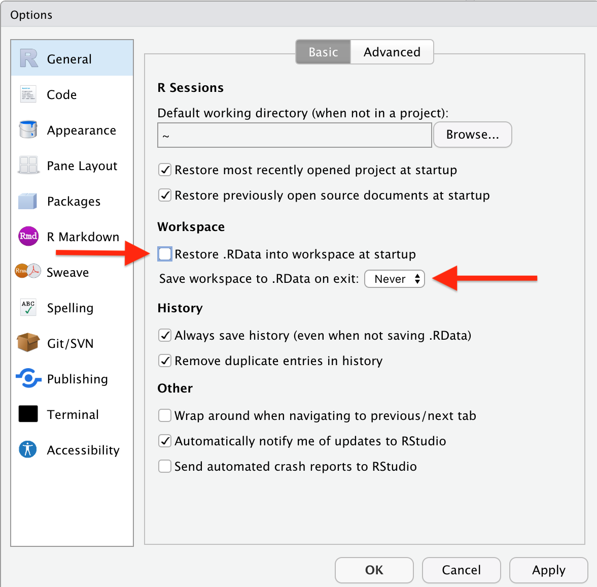
Practice good housekeeping to avoid unforeseen challenges down the road. If you create an R object worth saving, capture the R code that generated the object in an R script file. Save the R script, but don’t save the environment, or workspace, where the object was created.

To prevent RStudio from saving your workspace, open Preferences > General and un-select the option to restore .RData into workspace at startup. Be sure to specify that you never want to save your workspace, like this:

Now, each time you open RStudio, you will begin with an empty session. None of the code generated from your previous sessions will be remembered. The R script and datasets can be used to recreate the environment from scratch.

Other experts agree that not saving your workspace is best practice when using RStudio.

13. R Scripts

As we worked through this tutorial, we wrote code in the Console. As our projects become more complex, we write longer blocks of code. If we want to save our work, it is necessary to organize our code into a script. This allows us to keep track of our work on a project, write clean code with plenty of notes, reproduce our work, and share it with others.

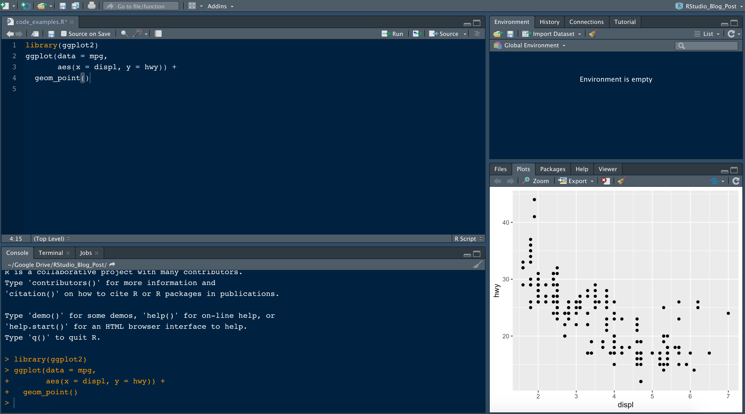
In RStudio, we can write scripts in the text editor window at the top left of the interface:

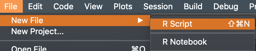
To create a new script, we can use the commands in the file menu:

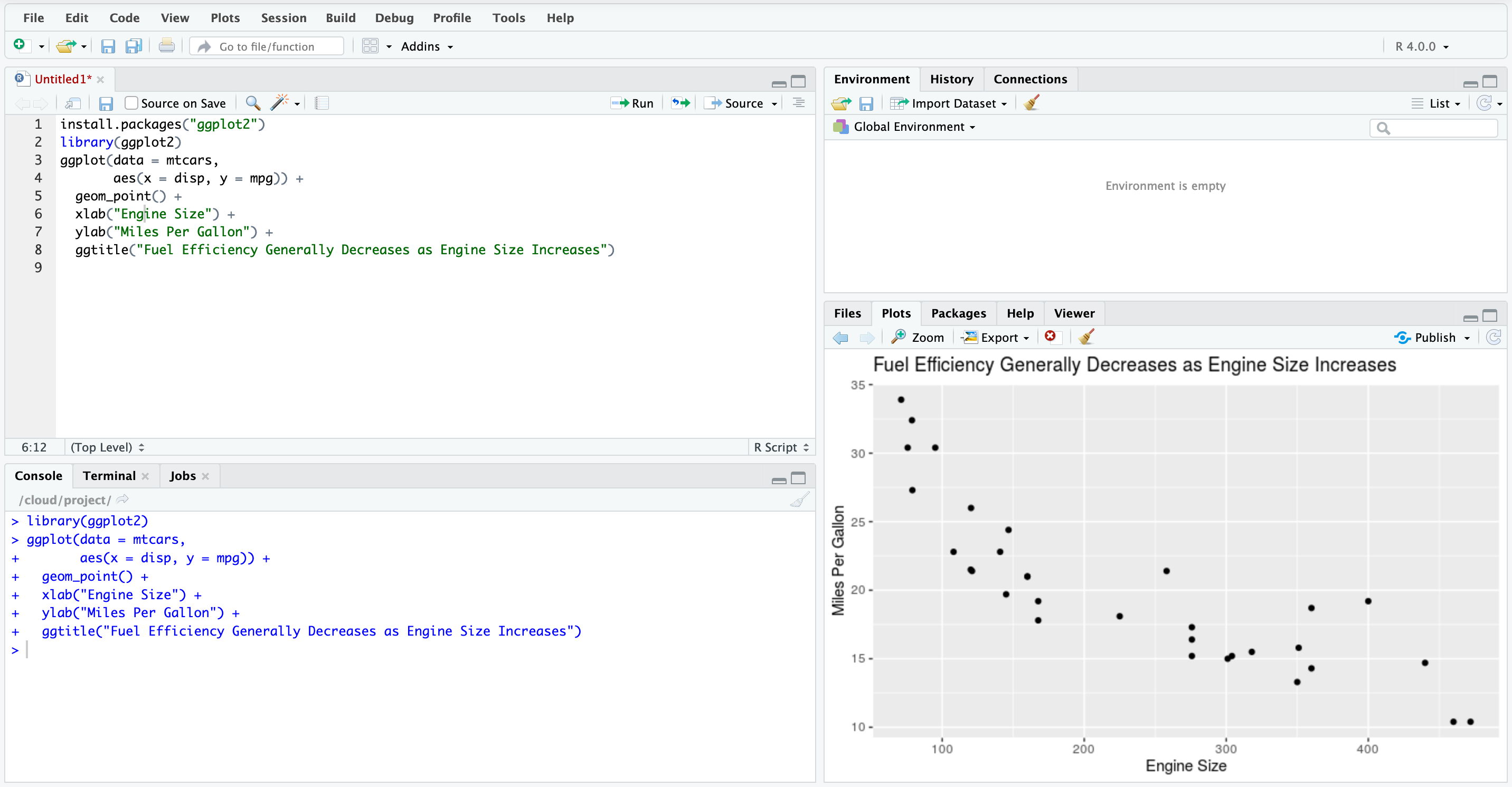
We can also use the keyboard shortcut Ctrl + Shift + N. When we save a script, it has the file extension .R. As an example, we’ll create a new script that includes this code to generate a scatterplot:

library(ggplot2)
ggplot(data = mpg,
       aes(x = displ, y = hwy)) +
  geom_point()

To save our script we navigate to the File menu tab and select Save. Or we enter the following command:

• Mac OS X: Cmd + S
• Windows/Linux: Ctrl + S

14. Run Code

To run a single line of code we typed into our script, we can either click Run at the top right of the script, or use the following keyboard commands when our cursor is on the line we want to run:

• Mac OS X: Cmd + Enter
• Windows/Linux: Ctrl + Enter

In this case, we’ll need to highlight multiple lines of code to generate the scatterplot. To highlight and run all lines of code in a script enter:

• Mac OS X: Cmd + A + Enter
• Windows/Linux: Ctrl + A + Enter

Let’s check out the result when we run the lines of code specified above:

Side note: this scatterplot is generated using data from the mpg dataset that is included in the ggplot2 package. The dataset contains fuel economy data from 1999 to 2008, for 38 popular models of cars.

In this plot, the engine displacement (i.e. size) is depicted on the x-axis (horizontal axis). The y-axis (vertical axis) depicts the fuel efficiency in miles-per-gallon. In general, fuel economy decreases with the increase in engine size. This plot was generated with the tidyverse package ggplot2. This package is very popular for data visualization in R.

15. Access Built-in Datasets

Want to learn more about the mpg dataset from the ggplot2 package that we mentioned in the last example? Do this with the following command:

data(mpg, package = "ggplot2")

From there you can take a look at the first six rows of data with the head() function:

head(mpg)
## # A tibble: 6 x 11
##   manufacturer model displ  year   cyl trans      drv     cty   hwy fl    class 
##   <chr>        <chr> <dbl> <int> <int> <chr>      <chr> <int> <int> <chr> <chr> 
## 1 audi         a4      1.8  1999     4 auto(l5)   f        18    29 p     compa…
## 2 audi         a4      1.8  1999     4 manual(m5) f        21    29 p     compa…
## 3 audi         a4      2    2008     4 manual(m6) f        20    31 p     compa…
## 4 audi         a4      2    2008     4 auto(av)   f        21    30 p     compa…
## 5 audi         a4      2.8  1999     6 auto(l5)   f        16    26 p     compa…
## 6 audi         a4      2.8  1999     6 manual(m5) f        18    26 p     compa…

Obtain summary statistics with the summary() function:

summary(mpg)
##  manufacturer          model               displ            year     
##  Length:234         Length:234         Min.   :1.600   Min.   :1999  
##  Class :character   Class :character   1st Qu.:2.400   1st Qu.:1999  
##  Mode  :character   Mode  :character   Median :3.300   Median :2004  
##                                        Mean   :3.472   Mean   :2004  
##                                        3rd Qu.:4.600   3rd Qu.:2008  
##                                        Max.   :7.000   Max.   :2008  
##       cyl           trans               drv                 cty       
##  Min.   :4.000   Length:234         Length:234         Min.   : 9.00  
##  1st Qu.:4.000   Class :character   Class :character   1st Qu.:14.00  
##  Median :6.000   Mode  :character   Mode  :character   Median :17.00  
##  Mean   :5.889                                         Mean   :16.86  
##  3rd Qu.:8.000                                         3rd Qu.:19.00  
##  Max.   :8.000                                         Max.   :35.00  
##       hwy             fl               class          
##  Min.   :12.00   Length:234         Length:234        
##  1st Qu.:18.00   Class :character   Class :character  
##  Median :24.00   Mode  :character   Mode  :character  
##  Mean   :23.44                                        
##  3rd Qu.:27.00                                        
##  Max.   :44.00

Or open the help page in the Help tab, like this:

help(mpg)

Finally, there are many datasets built-in to R that are ready to work with. Built-in datasets are handy for practicing new R skills without searching for data. View available datasets with this command:

data()

16. Style

When writing an R script, it’s good practice to specify packages to load at the top of the script:

library(ggplot2)

As we write R scripts, it’s also good practice add comments to explain our code (# like this). R ignores lines of code that begin with #. It’s common to share code with colleagues and collaborators. Ensuring they understand our methods will be very important. But more importantly, thorough notes are helpful to your future-self, so that you can understand your methods when you revisit the script in the future!

Here’s an example of what comments look like with our scatterplot code:

library(ggplot2)

# fuel economy data from 1999 to 2008, for 38 popular models of cars
# engine displacement (size) is depicted on the x-axis
# fuel efficiency is depicted on the y-axis
ggplot(data = mpg,
       aes(x = displ, y = hwy)) +
  geom_point()

17. Reproducible Reports with R Markdown

The comments used in the example above are fine for providing brief notes about our R script, but this format is not suitable for authoring reports where we need to summarize results and findings. We can author nicely formatted reports in RStudio using R Markdown files.

R Markdown is an open-source tool for producing reproducible reports in R. R Markdown enables us to keep all of our code, results, and writing, in one place. With R Markdown we have the option to export our work to numerous formats including PDF, Microsoft Word, a slideshow, or an html document for use in a website.

If you would like to learn R Markdown, check out these Dataquest blog posts:

• Getting Started with R Markdown — Guide and Cheatsheet
• R Markdown Tips, Tricks, and Shortcuts

18. Use RStudio Cloud

RStudio now offers a cloud-based version of RStudio Desktop called RStudio Cloud. RStudio Cloud allows you to code in RStudio without installing software, you only need a web browser. Almost everything we’ve learned in this tutorial applies to RStudio Cloud!

Work in RStudio Cloud is organized into projects similar to the desktop version. RStudio Cloud enables you to specify the version of R you wish to use for each project. This is great if you are revisiting an older project built around a previous version of R.

RStudio Cloud also makes it easy and secure to share projects with colleagues, and ensures that the working environment is fully reproducible every time the project is accessed.

The layout of RStudio Cloud is very similar to RStudio Desktop:

19. Get Your Hands Dirty!

The best way to learn RStudio is to apply what we’ve covered in this tutorial. Jump in on your own and familiarize yourself with RStudio! Create your own projects, save your work, and share your results. We can’t emphasize the importance of this enough.

Not sure where to start? Check out the additional resources listed below!

Additional Resources

If you enjoyed this tutorial, come learn with us at Dataquest! If you are new to R and RStudio, we recommend starting with the Dataquest Introduction to Data Analysis in R course. This is the first course in the Dataquest Data Analyst in R path.

For more advanced RStudio tips check out the Dataquest blog post 23 RStudio Tips, Tricks, and Shortcuts.

Learn how to load and clean data with tidyverse tools in this Dataquest blog post.

RStudio has published numerous in-depth how to articles about using RStudio. Find them here.

There is an official RStudio Blog.

If you would like to learn R Markdown, check out these Dataquest blog posts:

• Getting Started with R Markdown — Guide and Cheatsheet
• R Markdown Tips, Tricks, and Shortcuts

Learn R and the tidyverse with R for Data Science by Hadley Wickham. Solidify your knowledge by working through the exercises in RStudio and saving your work for future reference.

Bonus: Cheatsheets

RStudio has published numerous cheatsheets for working with R, including a detailed cheatsheet on using RStudio! Select cheatsheets can be accessed from within RStudio by selecting Help > Cheatsheets.

Casey is passionate about working with data, and is the R Team Lead at Dataquest. In his free time he enjoys outdoor adventures with his wife and kids.

The post Tutorial: Getting Started with R and RStudio appeared first on Dataquest.

In this tutorial we’ll learn how to begin programming with R using RStudio. We’ll install R, and RStudio RStudio, an extremely popular development environment for R. We’ll learn the key RStudio features in order to start programming in R on our own.

If you already know how to use RStudio and want to learn some tips, tricks, and shortcuts, check out this Dataquest blog post.

Table of Contents

• 1. Install R
• 2. Install RStudio
• 3. First Look at RStudio
• 4. The Console
• 5. The Global Environment
• 6. Install the tidyverse Packages
• 7. Load the tidyverse Packages into Memory
• 8. Identify Loaded Packages
• 9. Get Help on a Package
• 10. Get Help on a Function
• 11. RStudio Projects
• 12. Save Your “Real” Work. Delete the Rest.
• 13. R Scripts
• 14. Run Code
• 15. Access Built-in Datasets
• 16. Style
• 17. Reproducible Reports with R Markdown
• 18. Use RStudio Cloud
• 19. Get Your Hands Dirty!
• Additional Resources
• Bonus: Cheatsheets

Getting Started with RStudio

RStudio is an open-source tool for programming in R. RStudio is a flexible tool that helps you create readable analyses, and keeps your code, images, comments, and plots together in one place. It’s worth knowing about the capabilities of RStudio for data analysis and programming in R.

Using RStudio for data analysis and programming in R provides many advantages. Here are a few examples of what RStudio provides:

• An intuitive interface that lets us keep track of saved objects, scripts, and figures
• A text editor with features like color-coded syntax that helps us write clean scripts
• Auto complete features save time
• Tools for creating documents containing a project’s code, notes, and visuals
• Dedicated Project folders to keep everything in one place

RStudio can also be used to program in other languages including SQL, Python, and Bash, to name a few.

But before we can install RStudio, we’ll need to have a recent version of R installed on our computer.

1. Install R

R is available to download from the official R website. Look for this section of the web page:

The version of R to download depends on our operating system. Below, we include installation instructions for Mac OS X, Windows, and Linux (Ubuntu).

MAC OS X

• Select the Download R for (Mac) OSX option.
• Look for the most up-to-date version of R (new versions are released frequently and appear toward the top of the page) and click the .pkg file to download.
• Open the .pkg file and follow the standard instructions for installing applications on MAC OS X.
• Drag and drop the R application into the Applications folder.

Windows

• Select the Download R for Windows option.
• Select base, since this is our first installation of R on our computer.
• Follow the standard instructions for installing programs for Windows. If we are asked to select Customize Startup or Accept Default Startup Options, choose the default options.

Linux/Ubuntu

• Select the Download R for Linux option.
• Select the Ubuntu option.
• Alternatively, select the Linux package management system relevant to you if you are not using Ubuntu.

RStudio is compatible with many versions of R (R version 3.0.1 or newer as of July, 2020). Installing R separately from RStudio enables the user to select the version of R that fits their needs.

2. Install RStudio

Now that R is installed, we can install RStudio. Navigate to the RStudio downloads page.

When we reach the RStudio downloads page, let’s click the “Download” button of the RStudio Desktop Open Source License Free option:

Our operating system is usually detected automatically and so we can directly download the correct version for our computer by clicking the “Download RStudio” button. If we want to download RStudio for another operating system (other than the one we are running), navigate down to the “All installers” section of the page.

3. First Look at RStudio

When we open RStudio for the first time, we’ll probably see a layout like this:

But the background color will be white, so don’t expect to see this blue-colored background the first time RStudio is launched. Check out this Dataquest blog to learn how to customize the appearance of RStudio.

When we open RStudio, R is launched as well. A common mistake by new users is to open R instead of RStudio. To open RStudio, search for RStudio on the desktop, and pin the RStudio icon to the preferred location (e.g. Desktop or toolbar).

4. The Console

Let’s start off by introducing some features of the Console. The Console is a tab in RStudio where we can run R code.

Notice that the window pane where the console is located contains three tabs: Console, Terminal and Jobs (this may vary depending on the version of RStudio in use). We’ll focus on the Console for now.

When we open RStudio, the console contains information about the version of R we’re working with. Scroll down, and try typing a few expressions like this one. Press the enter key to see the result.

1 + 2

As we can see, we can use the console to test code immediately. When we type an expression like 1 + 2, we’ll see the output below after hitting the enter key.

We can store the output of this command as a variable. Here, we’ve named our variable result:

result <- 1 + 2

The <- is called the assignment operator. This operator assigns values to variables. The command above is translated into a sentence as:

> The result variable gets the value of one plus two.

One nice feature from RStudio is the keyboard shortcut for typing the assignment operator <-:

• Mac OS X: Option + -
• Windows/Linux: Alt + -

We highly recommend that you memorize this keyboard shortcut because it saves a lot of time in the long run!

When we type result into the console and hit enter, we see the stored value of 3:

> result <- 1 + 2
> result
[1] 3

When we create a variable in RStudio, it saves it as an object in the R global environment. We’ll discuss the environment and how to view objects stored in the environment in the next section.

5. The Global Environment

We can think of the global environment as our workspace. During a programming session in R, any variables we define, or data we import and save in a dataframe, are stored in our global environment. In RStudio, we can see the objects in our global environment in the Environment tab at the top right of the interface:

We’ll see any objects we created, such as result, under values in the Environment tab. Notice that the value, 3, stored in the variable is displayed.

Sometimes, having too many named objects in the global environment creates confusion. Maybe we’d like to remove all or some of the objects. To remove all objects, click the broom icon at the top of the window:

To remove selected objects from the workspace, select the Grid view from the dropdown menu:

Here we can check the boxes of the objects we’d like to remove and use the broom icon to clear them from our Global Environment.

6. Install the tidyverse Packages

Much of the functionality in R comes from using packages. Packages are shareable collections of code, data, and documentation. Packages are essentially extensions, or add-ons, to the R program that we installed above.

One of the most popular collection of packages in R is known as the “tidyverse”. The tidyverse is a collection of R packages designed for working with data. The tidyverse packages share a common design philosophy, grammar, and data structures. Tidyverse packages “play well together”. The tidyverse enables you to spend less time cleaning data so that you can focus more on analyzing, visualizing, and modeling data.

Let’s learn how to install the tidyverse packages. The most common “core” tidyverse packages are:

• readr, for data import.
• ggplot2, for data visualization.
• dplyr, for data manipulation.
• tidyr, for data tidying.
• purrr, for functional programming.
• tibble, for tibbles, a modern re-imagining of dataframes.
• stringr, for string manipulation.
• forcats, for working with factors (categorical data).

To install packages in R we use the built-in install.packages() function. We could install the packages listed above one-by-one, but fortunately the creators of the tidyverse provide a way to install all these packages from a single command. Type the following command in the Console and hit the enter key.

install.packages("tidyverse")

The install.packages() command only needs to be used to download and install packages for the first time.

7. Load the tidyverse Packages into Memory

After a package is installed on a computer’s hard drive, the library() command is used to load a package into memory:

library(readr)
library(ggplot2)

Loading the package into memory with library() makes the functionality of a given package available for use in the current R session. It is common for R users to have hundreds of R packages installed on their hard drive, so it would be inefficient to load all packages at once. Instead, we specify the R packages needed for a particular project or task.

Fortunately, the core tidyverse packages can be loaded into memory with a single command. This is how the command and the output looks in the console:

library(tidyverse)## ── Attaching packages ───────────────────────────────────────────────── tidyverse 1.3.0 ──## ✓ ggplot2 3.3.2 ✓ purrr 0.3.4
## ✓ tibble 3.0.3 ✓ dplyr 1.0.0
## ✓ tidyr 1.1.0 ✓ stringr 1.4.0
## ✓ readr 1.3.1 ✓ forcats 0.5.0## ── Conflicts ──────────────────────────────────────────────────── tidyverse_conflicts() ──
## x dplyr::filter() masks stats::filter()
## x dplyr::lag() masks stats::lag()

The Attaching packages section of the output specifies the packages and their versions loaded into memory. The Conflicts section specifies any function names included in the packages that we just loaded to memory that share the same name as a function already loaded into memory. Using the example above, now if we call the filter() function, R will use the code specified for this function from the dplyr package. These conflicts are generally not a problem, but it’s worth reading the output message to be sure.

8. Identify Loaded Packages

If we need to check which packages we loaded, we can refer to the Packages tab in the window at the bottom right of the console.

We can search for packages, and checking the box next to a package loads it (the code appears in the console).

Alternatively, entering this code into the console will display all packages currently loaded into memory:

(.packages())

Which returns:

[1] "forcats" "stringr" "dplyr" "purrr" "tidyr" "tibble" "tidyverse"
[8] "ggplot2" "readr" "stats" "graphics" "grDevices" "utils" "datasets" 
[15] "methods" "base"

Another useful function for returning the names of packages currently loaded into memory is search():

> search()
 [1] ".GlobalEnv" "package:forcats" "package:stringr" "package:dplyr" 
 [5] "package:purrr" "package:readr" "package:tidyr" "package:tibble" 
 [9] "package:ggplot2" "package:tidyverse" "tools:rstudio" "package:stats" 
[13] "package:graphics" "package:grDevices" "package:utils" "package:datasets" 
[17] "package:methods" "Autoloads" "package:base"

9. Get Help on a Package

We’ve learned how to install and load packages. But what if we’d like to learn more about a package that we’ve installed? That’s easy! Clicking the package name in the Packages tab takes us to the Help tab for the selected package. Here’s what we see if we click the tidyr package:

Alternatively, we can type this command into the console and achieve the same result:

help(package = "tidyr")

The help page for a package provides quick access to documentation for each function included in a package. From the main help page for a package you can also access “vignettes” when they are available. Vignettes provide brief introductions, tutorials, or other reference information about a package, or how to use specific functions in a package.

vignette(package = "tidyr")

Which results in this list of available options:

Vignettes in package ‘tidyr’:nest nest (source, html)
pivot Pivoting (source, html)
programming Programming with tidyr (source, html)
rectangle rectangling (source, html)
tidy-data Tidy data (source, html)
in-packages Usage and migration (source, html)

From there, we can select a particular vignette to view:

vignette("pivot")

Now we see the Pivot vignette is displayed in the Help tab. This is one example of why RStudio is a powerful tool for programming in R. We can access function and package documentation and tutorials without leaving RStudio!

10. Get Help on a Function

As we learned in the last section, we can get help on a function by clicking the package name in Packages and then click on a function name to see the help file. Here we see the pivot_longer() function from the tidyr package is at the top of this list:

And if we click on “pivot_longer” we get this: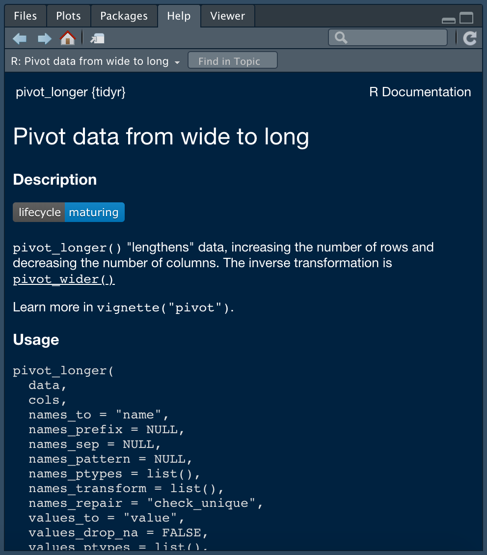

We can achieve the same results in the Console with any of these function calls:

help("pivot_longer")
help(pivot_longer)
?pivot_longer

Note that the specific Help tab for the pivot_longer() function (or any function we’re interested in) may not be the default result if the package that contains the function is not loaded into memory yet. In general it’s best to ensure a specific package is loaded before seeking help on a function.

11. RStudio Projects

RStudio offers a powerful feature to keep you organized; Projects. It is important to stay organized when you work on multiple analyses. Projects from RStudio allow you to keep all of your important work in one place, including code scripts, plots, figures, results, and datasets.

Create a new project by navigating to the File tab in RStudio and select New Project.... Then specify if you would like to create the project in a new directory, or in an existing directory. Here we select “New Directory”:

RStudio offers dedicated project types if you are working on an R package, or a Shiny Web Application. Here we select “New Project”, which creates an R project:

Next, we give our project a name. “Create project as a subdirectory of:” is showing where the folder will live on the computer. If we approve of the location select “Create Project”, if we do not, select “Browse” and choose the location on the computer where this project folder should live.

Now in RStudio we see the name of the project is indicated in the upper-right corner of the screen. We also see the .Rproj file in the Files tab. Any files we add to, or generate-within, this project will appear in the Files tab.

RStudio Projects are useful when you need to share your work with colleagues. You can send your project file (ending in .Rproj) along with all supporting files, which will make it easier for your colleagues to recreate the working environment and reproduce the results.

12. Save Your “Real” Work. Delete the Rest.

This tip comes from our 23 RStudio Tips, Tricks, and Shortcuts blog post, but it’s so important that we are sharing it here as well!

Practice good housekeeping to avoid unforeseen challenges down the road. If you create an R object worth saving, capture the R code that generated the object in an R script file. Save the R script, but don’t save the environment, or workspace, where the object was created.

To prevent RStudio from saving your workspace, open Preferences > General and un-select the option to restore .RData into workspace at startup. Be sure to specify that you never want to save your workspace, like this:

Now, each time you open RStudio, you will begin with an empty session. None of the code generated from your previous sessions will be remembered. The R script and datasets can be used to recreate the environment from scratch.

Other experts agree that not saving your workspace is best practice when using RStudio.

13. R Scripts

As we worked through this tutorial, we wrote code in the Console. As our projects become more complex, we write longer blocks of code. If we want to save our work, it is necessary to organize our code into a script. This allows us to keep track of our work on a project, write clean code with plenty of notes, reproduce our work, and share it with others.

In RStudio, we can write scripts in the text editor window at the top left of the interface:

To create a new script, we can use the commands in the file menu:

We can also use the keyboard shortcut Ctrl + Shift + N. When we save a script, it has the file extension .R. As an example, we’ll create a new script that includes this code to generate a scatterplot:

library(ggplot2)
ggplot(data = mpg,
       aes(x = displ, y = hwy)) +
  geom_point()

To save our script we navigate to the File menu tab and select Save. Or we enter the following command:

• Mac OS X: Cmd + S
• Windows/Linux: Ctrl + S

14. Run Code

To run a single line of code we typed into our script, we can either click Run at the top right of the script, or use the following keyboard commands when our cursor is on the line we want to run:

• Mac OS X: Cmd + Enter
• Windows/Linux: Ctrl + Enter

In this case, we’ll need to highlight multiple lines of code to generate the scatterplot. To highlight and run all lines of code in a script enter:

• Mac OS X: Cmd + A + Enter
• Windows/Linux: Ctrl + A + Enter

Let’s check out the result when we run the lines of code specified above:

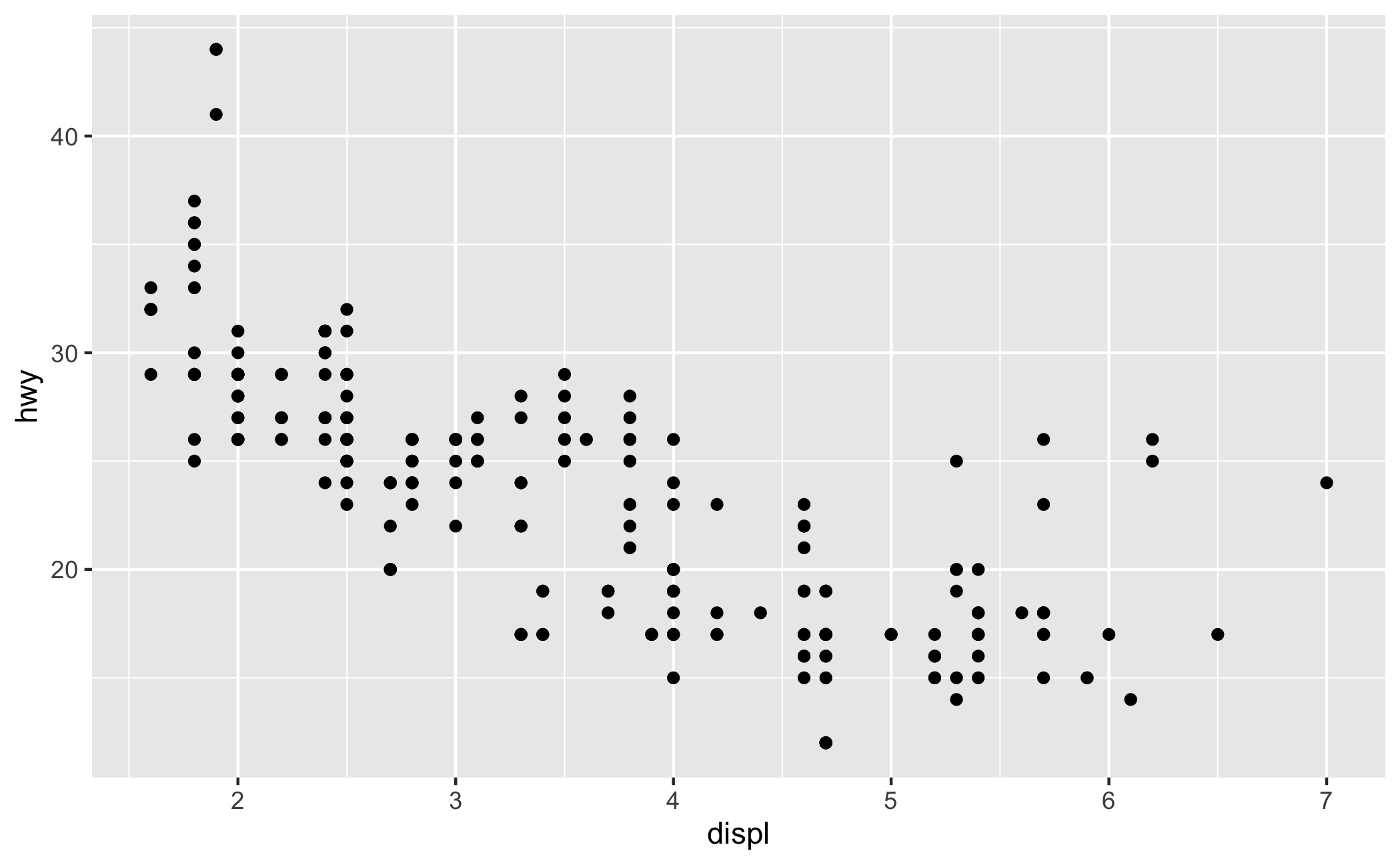
Side note: this scatterplot is generated using data from the mpg dataset that is included in the ggplot2 package. The dataset contains fuel economy data from 1999 to 2008, for 38 popular models of cars.

In this plot, the engine displacement (i.e. size) is depicted on the x-axis (horizontal axis). The y-axis (vertical axis) depicts the fuel efficiency in miles-per-gallon. In general, fuel economy decreases with the increase in engine size. This plot was generated with the tidyverse package ggplot2. This package is very popular for data visualization in R.

15. Access Built-in Datasets

Want to learn more about the mpg dataset from the ggplot2 package that we mentioned in the last example? Do this with the following command:

data(mpg, package = "ggplot2")

From there you can take a look at the first six rows of data with the head() function:

head(mpg)

## # A tibble: 6 x 11
##   manufacturer model displ  year   cyl trans      drv     cty   hwy fl    class 
##                          
## 1 audi         a4      1.8  1999     4 auto(l5)   f        18    29 p     compa…
## 2 audi         a4      1.8  1999     4 manual(m5) f        21    29 p     compa…
## 3 audi         a4      2    2008     4 manual(m6) f        20    31 p     compa…
## 4 audi         a4      2    2008     4 auto(av)   f        21    30 p     compa…
## 5 audi         a4      2.8  1999     6 auto(l5)   f        16    26 p     compa…
## 6 audi         a4      2.8  1999     6 manual(m5) f        18    26 p     compa…

Obtain summary statistics with the summary() function:

summary(mpg)

##  manufacturer          model               displ            year     
##  Length:234         Length:234         Min.   :1.600   Min.   :1999  
##  Class :character   Class :character   1st Qu.:2.400   1st Qu.:1999  
##  Mode  :character   Mode  :character   Median :3.300   Median :2004  
##                                        Mean   :3.472   Mean   :2004  
##                                        3rd Qu.:4.600   3rd Qu.:2008  
##                                        Max.   :7.000   Max.   :2008  
##       cyl           trans               drv                 cty       
##  Min.   :4.000   Length:234         Length:234         Min.   : 9.00  
##  1st Qu.:4.000   Class :character   Class :character   1st Qu.:14.00  
##  Median :6.000   Mode  :character   Mode  :character   Median :17.00  
##  Mean   :5.889                                         Mean   :16.86  
##  3rd Qu.:8.000                                         3rd Qu.:19.00  
##  Max.   :8.000                                         Max.   :35.00  
##       hwy             fl               class          
##  Min.   :12.00   Length:234         Length:234        
##  1st Qu.:18.00   Class :character   Class :character  
##  Median :24.00   Mode  :character   Mode  :character  
##  Mean   :23.44                                        
##  3rd Qu.:27.00                                        
##  Max.   :44.00

Or open the help page in the Help tab, like this:

help(mpg)

Finally, there are many datasets built-in to R that are ready to work with. Built-in datasets are handy for practicing new R skills without searching for data. View available datasets with this command:

data()

16. Style

When writing an R script, it’s good practice to specify packages to load at the top of the script:

library(ggplot2)

As we write R scripts, it’s also good practice add comments to explain our code (# like this). R ignores lines of code that begin with #. It’s common to share code with colleagues and collaborators. Ensuring they understand our methods will be very important. But more importantly, thorough notes are helpful to your future-self, so that you can understand your methods when you revisit the script in the future!

Here’s an example of what comments look like with our scatterplot code:

library(ggplot2)

# fuel economy data from 1999 to 2008, for 38 popular models of cars
# engine displacement (size) is depicted on the x-axis
# fuel efficiency is depicted on the y-axis
ggplot(data = mpg,
       aes(x = displ, y = hwy)) +
  geom_point()

17. Reproducible Reports with R Markdown

The comments used in the example above are fine for providing brief notes about our R script, but this format is not suitable for authoring reports where we need to summarize results and findings. We can author nicely formatted reports in RStudio using R Markdown files.

R Markdown is an open-source tool for producing reproducible reports in R. R Markdown enables us to keep all of our code, results, and writing, in one place. With R Markdown we have the option to export our work to numerous formats including PDF, Microsoft Word, a slideshow, or an html document for use in a website.

If you would like to learn R Markdown, check out these Dataquest blog posts:

• Getting Started with R Markdown — Guide and Cheatsheet
• R Markdown Tips, Tricks, and Shortcuts

18. Use RStudio Cloud

RStudio now offers a cloud-based version of RStudio Desktop called RStudio Cloud. RStudio Cloud allows you to code in RStudio without installing software, you only need a web browser. Almost everything we’ve learned in this tutorial applies to RStudio Cloud!

Work in RStudio Cloud is organized into projects similar to the desktop version. RStudio Cloud enables you to specify the version of R you wish to use for each project. This is great if you are revisiting an older project built around a previous version of R.

RStudio Cloud also makes it easy and secure to share projects with colleagues, and ensures that the working environment is fully reproducible every time the project is accessed.

The layout of RStudio Cloud is very similar to RStudio Desktop:

19. Get Your Hands Dirty!

The best way to learn RStudio is to apply what we’ve covered in this tutorial. Jump in on your own and familiarize yourself with RStudio! Create your own projects, save your work, and share your results. We can’t emphasize the importance of this enough.

Not sure where to start? Check out the additional resources listed below!

Additional Resources

If you enjoyed this tutorial, come learn with us at Dataquest! If you are new to R and RStudio, we recommend starting with the Dataquest Introduction to Data Analysis in R course. This is the first course in the Dataquest Data Analyst in R path.

For more advanced RStudio tips check out the Dataquest blog post 23 RStudio Tips, Tricks, and Shortcuts.

Learn how to load and clean data with tidyverse tools in this Dataquest blog post.

RStudio has published numerous in-depth how to articles about using RStudio. Find them here.

There is an official RStudio Blog.

If you would like to learn R Markdown, check out these Dataquest blog posts:

• Getting Started with R Markdown — Guide and Cheatsheet
• R Markdown Tips, Tricks, and Shortcuts

Learn R and the tidyverse with R for Data Science by Hadley Wickham. Solidify your knowledge by working through the exercises in RStudio and saving your work for future reference.

Bonus: Cheatsheets

RStudio has published numerous cheatsheets for working with R, including a detailed cheatsheet on using RStudio! Select cheatsheets can be accessed from within RStudio by selecting Help > Cheatsheets.