Project Jupyter’s tools are available for installation via the Python Package Index, the leading repository of software created for the Python programming language.
This page uses instructions with pip, the recommended installation tool for Python. If you require environment management as opposed to just installation, look into conda, mamba, pipenv, and Homebrew.
JupyterLab
Install JupyterLab with pip:
Note: If you install JupyterLab with conda or mamba, we recommend using the conda-forge channel.
Once installed, launch JupyterLab with:
Jupyter Notebook
Install the classic Jupyter Notebook with:
To run the notebook:
Voilà
Install Voilà with:
Once installed, launch Voilà with:
Homebrew
Homebrew is a package manager for macOS and Linux.
You can use it to install Jupyter by running:
Jupyter Notebook is an open-source web application that allows you to create and share documents that contain live code, equations, visualizations, and narrative text. Uses include data cleaning and transformation, numerical simulation, statistical modeling, data visualization, machine learning, and much more.
Jupyter has support for over 40 different programming languages and Python is one of them. Python is a requirement (Python 3.3 or greater, or Python 2.7) for installing the Jupyter Notebook itself.
Jupyter Notebook can be installed by using either of the two ways described below:
- Using Anaconda:
Install Python and Jupyter using the Anaconda Distribution, which includes Python, the Jupyter Notebook, and other commonly used packages for scientific computing and data science. To install Anaconda, go through How to install Anaconda on windows? and follow the instructions provided. -
Using PIP:
Install Jupyter using the PIP package manager used to install and manage software packages/libraries written in Python. To install pip, go through How to install PIP on Windows? and follow the instructions provided.
Installing Jupyter Notebook using Anaconda:
Anaconda is an open-source software that contains Jupyter, spyder, etc that are used for large data processing, data analytics, heavy scientific computing. Anaconda works for R and python programming language. Spyder(sub-application of Anaconda) is used for python. Opencv for python will work in spyder. Package versions are managed by the package management system called conda.
To install Jupyter using Anaconda, just go through the following instructions:
Launching Jupyter:
Installing Jupyter Notebook using pip:
PIP is a package management system used to install and manage software packages/libraries written in Python. These files are stored in a large “on-line repository” termed as Python Package Index (PyPI).
pip uses PyPI as the default source for packages and their dependencies.
To install Jupyter using pip, we need to first check if pip is updated in our system. Use the following command to update pip:
python -m pip install --upgrade pip
After updating the pip version, follow the instructions provided below to install Jupyter:
- Command to install Jupyter:
python -m pip install jupyter
- Beginning Installation:

- Downloading Files and Data:

- Installing Packages:

- Finished Installation:


Launching Jupyter:
Use the following command to launch Jupyter using command-line:
jupyter notebook

Last Updated :
05 Oct, 2021
Like Article
Save Article
Jupyter Notebook
This is a quick guide to install Jupyter Notebook with Conda and pip on Windows or Mac operating system. We’ll guide you through the installation process for both Mac and Windows operating systems.

Install Jupyter Notebook on Windows
Walk though of installing Jupyter on Windows using Anaconda, Miniconda and Pip.

Install Jupyter Notebook on Mac OS
Walk though of installing Jupyter on Mac using Anaconda, Miniconda and Pip.

Getting Started With Jupyter Notebook
Once you have Jupyter Notebook installed, you can start creating and editing notebooks.
Introduction: Jupyter Notebook and Python Environment Tools
Jupyter Notebook is an open-source, interactive web application that allows you to create, share, and collaborate on documents containing live code, equations, visualizations, and narrative text. It is widely used for data analysis, scientific computing, and teaching programming concepts. In this article, we’ll guide you through the installation process for both Mac and Windows operating systems.
| Option | Description |
|---|---|
Anaconda |
Anaconda is a free and open-source distribution of Python and R programming languages that includes a wide range of pre-installed packages and libraries, such as NumPy, pandas, and Jupyter Notebook, which makes it convenient for users who need a comprehensive environment for their projects. However, the full installation can require over 3 GB of disk space which includes an extensive list of pre-installed packages, saving saves time and effort in setting up a fully functional environment. |
Miniconda |
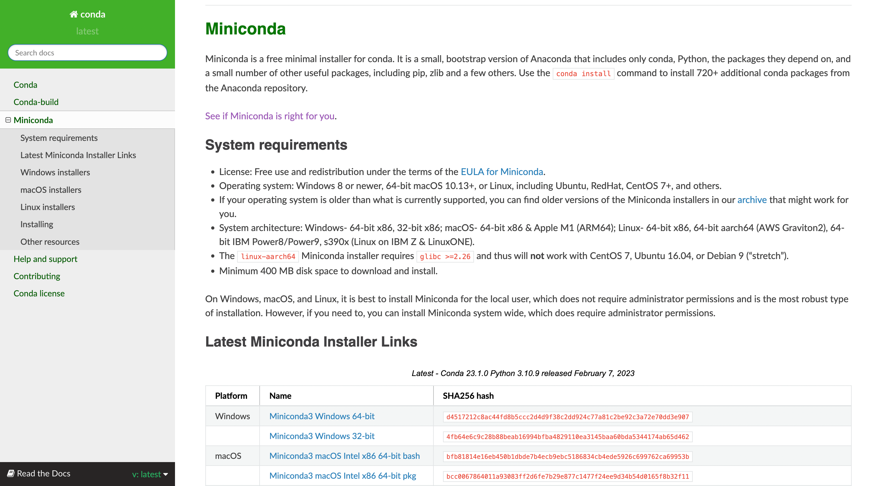
Miniconda is a lightweight version of Anaconda that provides a minimalistic Python environment, including only the necessary components to run Conda, the package, and environment manager. Unlike Anaconda, Miniconda does not include pre-installed packages. Users can install only the specific packages they need for their projects, which makes it a suitable choice for those who prefer a more compact and customizable environment. Miniconda has much lower memory requirements compared to Anaconda, taking up only 400-500 MB of disk space and making it an attractive option for users who prefer to manage their packages individually. |
Conda |
Conda is an open-source, cross-platform package manager and environment management system that is the core component of both Anaconda and Miniconda distributions. To use conda, we need to have either Anaconda or Miniconda. |
|
Pip |
Pip is the default package manager for Python that comes bundled with the standard Python distribution. Pip installs packages from the Python Package Index (PyPI) and is focused on managing packages specifically for the Python ecosystem. Pip lacks built-in support for managing environments. However, you can use it alongside Python’s built-in venv module to create isolated environments. It may be challenging to resolve and manage complex dependencies with pip, especially for packages with dependencies on non-Python libraries. |
What should I install, Anaconda, Conda, or Pip
Deciding what to install depends on your specific needs, requirements, and preferences. Here’s a brief comparison between Anaconda, Miniconda, and pip to help you make an informed decision.
| Option | Benefits | Choose If |
|---|---|---|
| Anaconda |
|
|
| Miniconda |
|
|
| Pip |
|
|
Choosing the right Python environment tool depends on individual needs and preferences.
Anaconda offers a comprehensive environment with over 3 GB of pre-installed packages, making it suitable for those seeking a straightforward installation for scientific computing. Miniconda provides a lightweight and minimalistic environment, allowing users to install only the packages they need, making it an attractive option for those with limited storage space. Pip, on the other hand, is the default Python package manager that appeals to those comfortable with a command-line interface and who prefer a more manual approach to package installation.
Understanding the benefits and use cases of Anaconda, Miniconda, and Pip helps users make an informed decision that aligns with their specific requirements for Python development, data science, or machine learning projects.
There are two main methods to install Jupyter Notebook on Windows: using Anaconda or pip. We’ll cover both methods in the following sections.
Installing Jupyter Notebook using Anaconda on Windows
Anaconda is a free, open-source Python distribution that includes many popular scientific computing and data science packages, including Jupyter Notebook.
Step 1: Download Anaconda
Visit the Anaconda distribution page and download the latest version for Windows.

Step 2: Run the Anaconda Installer
Run the downloaded executable file to start installing. Follow the on-screen instructions and accept the default settings.
Step 3: Launch Jupyter Notebook
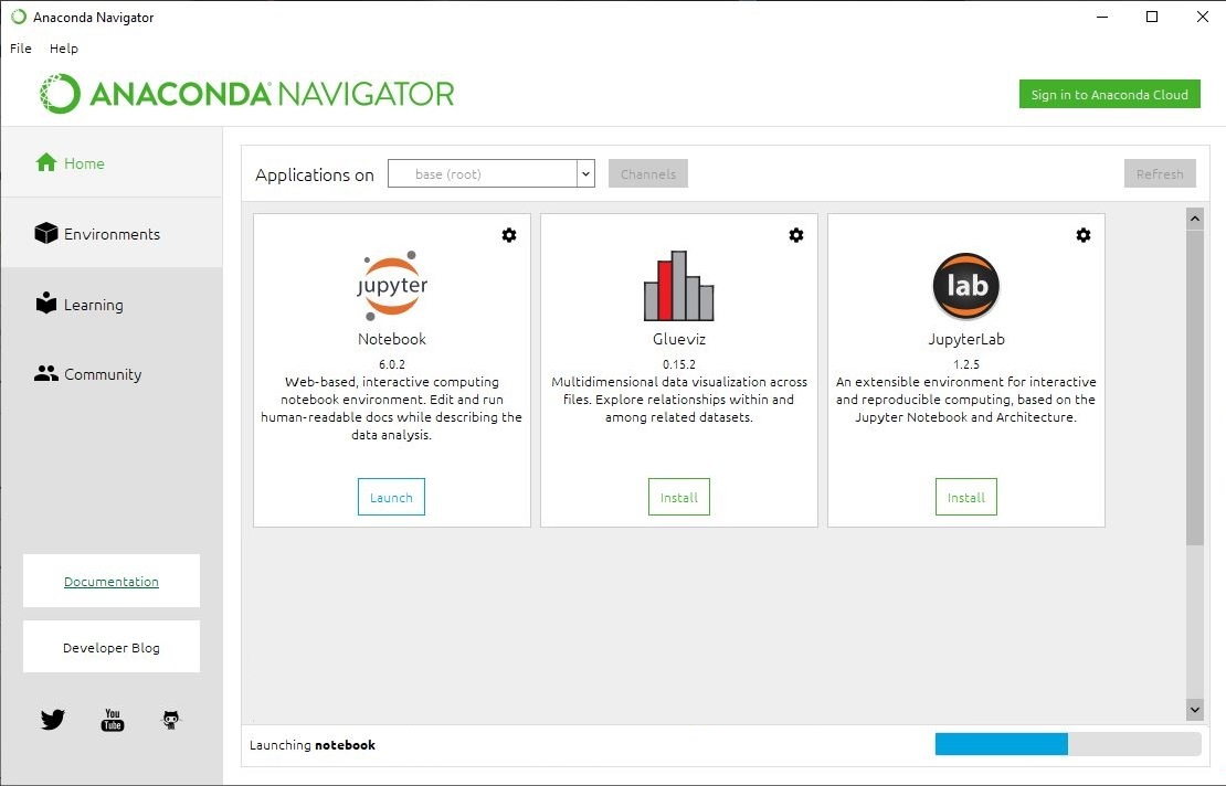
Once the installation is complete, launch Anaconda Navigator from the Start menu. Click on the Jupyter Notebook icon to launch the application.
Installing Jupyter Notebook using Miniconda on Windows
To install Jupyter Notebook using Miniconda on Windows, follow these steps:
Step 1: Download Miniconda
Visit the Miniconda download page and download the Miniconda installer for Windows. Choose the Python version you prefer (usually the latest version is recommended) and select the appropriate installer based on your system architecture (64-bit or 32-bit).
Step 2: Install Miniconda
Run the downloaded Miniconda installer (.exe file) by double-clicking it. Follow the installation prompts, and make sure to check the option “Add Miniconda to my PATH environment variable” during the installation. This ensures that Miniconda and its associated commands are accessible from the command line.
Step 3: Open Command Prompt or PowerShell
Press `Win + R`, type cmd or powershell, and press Enter to open the Command Prompt or PowerShell window.
Step 4: Update Conda
Before installing Jupyter Notebook, it is a good practice to update Conda to the latest version. Run the command to update Conda:
conda update -n base -c defaults conda
Step 5: Create a new Conda environment (optional)
It’s recommended to create a separate Conda environment for your project to avoid potential conflicts between packages. Replace myenv with your desired environment name and <python_version> with your preferred Python version (e.g., 3.9):
conda create -n myenv python=<python_version>Activate the newly created environment by running:
conda activate myenv
Step6: Install Jupyter Notebook
With Conda updated and your environment activated (if created), install Jupyter Notebook using the following command:
conda install -c conda-forge notebookThis command installs Jupyter Notebook from the conda-forge channel.
Step 6: Launch Jupyter Notebook
Start Jupyter Notebook by running this command:
jupyter notebookThis command will open Jupyter Notebook in your default web browser. You can now create, edit, and run Jupyter Notebooks within the specified Conda environment.
Jupyter Notebook Install Using pip on Windows
If you prefer not to use conda, you can install Jupyter Notebook using pip package manager for Python.
Step 1: Install Python programming language
Download and install the latest version of Python from the official website (https://www.python.org/downloads/). Make sure to check the option “Add Python to PATH” during the installation.
Step 2: Install Jupyter Notebook
Open the Command Prompt and run the following command using pip install to install Jupyter Notebook:
pip install jupyter
Step 3: Start Jupyter Notebook
Type the following command in the Command Prompt to launch Jupyter Notebook:
jupyter notebookHow to Install Jupyter Notebook on Mac
There are two main methods to install Jupyter Notebook on Mac: using Anaconda or pip. We’ll cover both methods in the following sections.
Installing Jupyter Notebook using Anaconda on Mac
The process of installing Jupyter Notebook using Anaconda on Mac is very similar to the Windows installation.
Step 1: Download Anaconda
Visit the Anaconda distribution page and download the latest version for macOS.
Step 2: Run the Anaconda Installer
Open the downloaded file and follow the on-screen instructions. Accept the default settings to complete the installation.
Step 3: Launch Jupyter Notebook
Open the Anaconda Navigator from your Applications folder. Click on the Jupyter Notebook icon to launch the application.
Jupyter Notebook Install Using `pip` on Mac
The process of installing Jupyter Notebook using pip on Mac is similar to the Windows installation.
Step 1: Install Python
Download and install the latest version of Python from the official website (https://www.python.org/downloads/).
Step 2: Install Jupyter Notebook
Open the Terminal and run the following command to install Jupyter Notebook:
pip3 install jupyterStep 3: Launch Jupyter Notebook
Type the following command in the Terminal to launch Jupyter Notebook:
jupyter notebookGetting Started With Jupyter Notebook
Now that you have Jupyter Notebook installed, you can start creating and editing notebooks.
Building your first Jupyter Notebook project
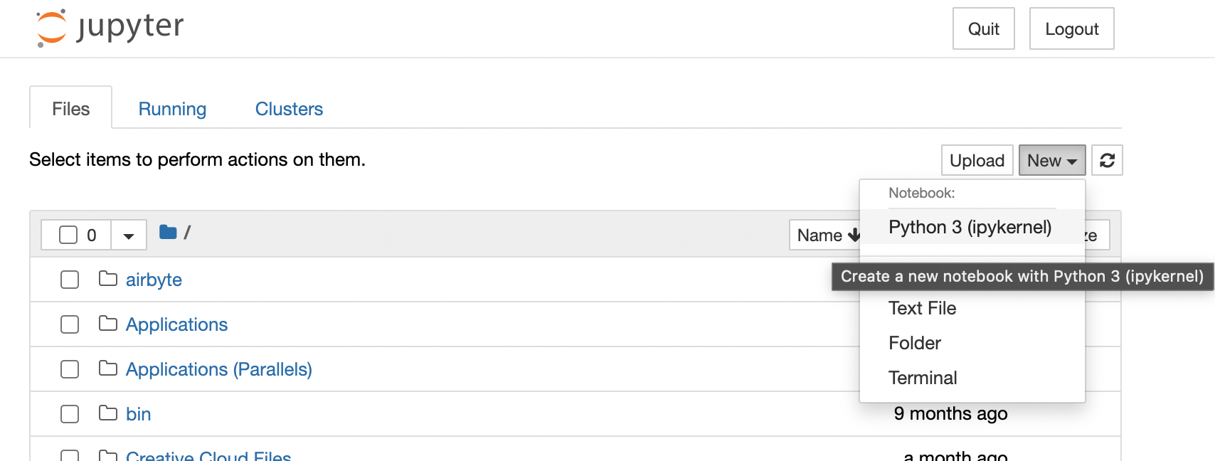
To create a new notebook, click on the “New” button in the top right corner of the Jupyter Notebook interface and select “Python 3” (or the version you have installed) from the drop-down menu.
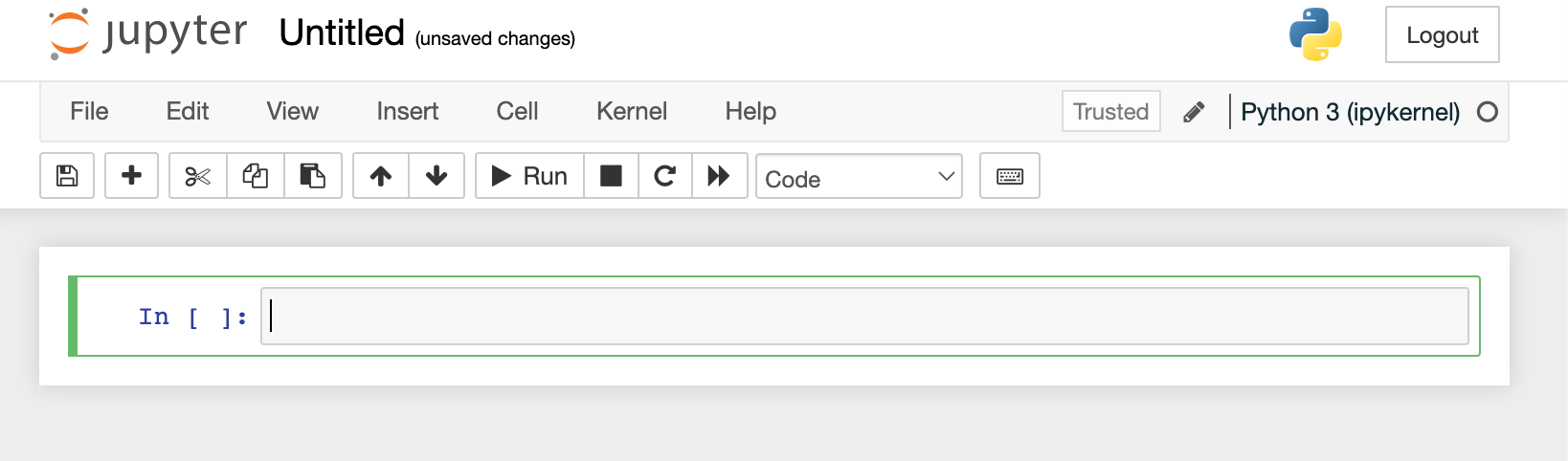
A new notebook will open with an empty code cell. You can start writing your code, markdown text, or equations in the cell. To execute the code in a cell, press Shift + Enter.
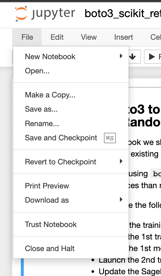
You can add new cells, delete cells, or change the cell type (code, markdown, or raw) using the toolbar at the top of the notebook. Additionally, you can access various notebook settings, download the notebook in different formats, or save and checkpoint your progress using the “File” and “Kernel” menus.
Installing a Python Module in Jupyter Notebook with pip install
To install additional Python modules in Jupyter, use the `!pip` or `!pip3` command followed by the module name. For example, to install the NumPy module, run the following command in a Jupyter Notebook cell:
!pip install numpyFor Mac users, you might need to use pip3:
!pip3 install numpy
Classic Jupyter Notebook is a powerful tool. However, if you are looking to collaborate with others in a seamless could based Notebook that supports simultaneous use of Python, R and SQL, check out Noteable. It is fully compatible with classic Jupyter notebook, meaning you can import and export `ipynb` files, and requires no set up at all. Just sign up and code away!
Все курсы > Программирование на Питоне > Занятие 14

Программа Jupyter Notebook — это локальная программа, которая открывается в браузере и позволяет интерактивно исполнять код на Питоне, записанный в последовательности ячеек.

Облачной версией Jupyter Notobook является программа Google Colab, которой мы уже давно пользуемся на курсах машинного обучения. Если вы проходили мои занятия, то в работе с этой программой для вас не будет почти ничего нового.
Способ 1. Если на вашем компьютере уже установлен Питон, то установить Jupyter Notebook можно через менеджер пакетов pip.
Способ 2 (рекомендуется). Кроме того, Jupyter Notebook входит в дистрибутив Питона под названием Anaconda.
На сегодняшнем занятии мы рассмотрим именно второй вариант установки.
Anaconda
Anaconda — это дистрибутив Питона и репозиторий пакетов, специально предназначенных для анализа данных и машинного обучения.
![]()
Основу дистрибутива Anaconda составляет система управления пакетами и окружениями conda.
Conda можно управлять двумя способами, а именно через Anaconda Prompt — программу, аналогичную командной строке Windows, или через Anaconda Navigator — понятный графический интерфейс.
Кроме того, в дистрибутив Anaconda входит несколько полезных программ:
- Jupyter Notebook и JupyterLab — это программы, позволяющие исполнять код на Питоне (и, как мы увидим, на других языках) и обрабатывать данные.
- Spyder и PyCharm представляют собой так называемую интегрированную среду разработки (Integrated Development Environment, IDE). IDE — это редактор кода наподобие программы Atom или Sublime Text с дополнительными возможностями автодополнения, компиляции и интерпретации, анализа ошибок, отладки (debugging), подключения к базам данных и др.
- RStudio — интегрированная среда разработки для программирования на R.
На схеме структура Anaconda выглядит следующим образом:

Установка дистрибутива Anaconda на Windows
Шаг 1. Скачайте Anaconda⧉ с официального сайта.
Шаг 2. Запустите установщик.
На одном из шагов установки вам предложат поставить две галочки, в частности (1) добавить Anaconda в переменную path и (2) сделать дистрибутив Anaconda версией, которую Windows обнаруживает по умолчанию.
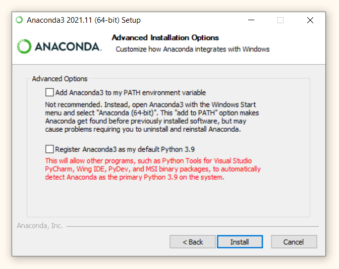
Не отмечайте ни один из пунктов!
Так вы сможете использовать два дистрибутива Питона, первый дистрибутив мы установили на прошлом занятии, второй — сейчас.
Как запустить Jupyter Notebook
После того как вы скачали и установили Anaconda, можно переходить к запуску ноутбука.
Шаг 1. Откройте Anaconda Navidator
Открыть Anaconda Navigator можно двумя способами.
Способ 1. Запуск из меню «Пуск». Просто перейдите в меню «Пуск» и выберите Anaconda Navigator.

Способ 2. Запуск через Anaconda Prompt. Также из меню «Пуск» откройте терминал Anaconda Prompt.

Введите команду
anaconda-navigator.
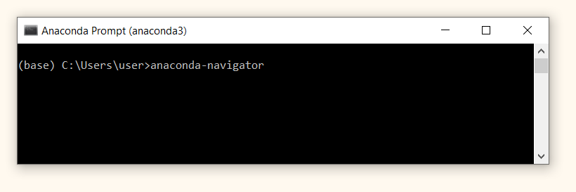
В результате должно появиться вот такое окно.
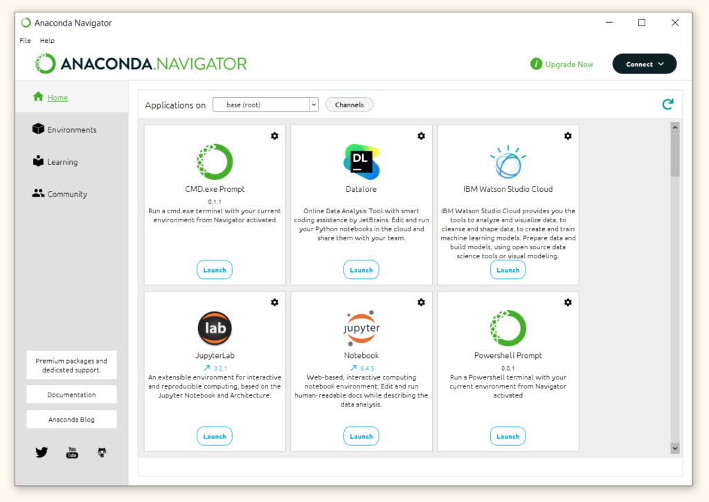
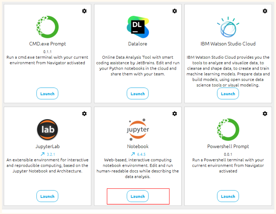
Шаг 2. Откройте Jupyter Notebook
Теперь выберите Jupyter Notebook и нажмите Launch («Запустить»).
Замечу, что Jupyter Notebook можно открыть не только из Anaconda Navigator, но и через меню «Пуск», а также введя в терминале Anaconda Prompt команду
jupyter-notebook.
В результате должен запуститься локальный сервер, и в браузере откроется перечень папок вашего компьютера.

Шаг 3. Выберите папку и создайте ноутбук
Выберите папку, в которой хотите создать ноутбук. В моем случае я выберу Рабочий стол (Desktop).
Теперь в правом верхнем углу нажмите New → Python 3.

Мы готовы писать и исполнять код точно также, как мы это делаем в Google Colab.
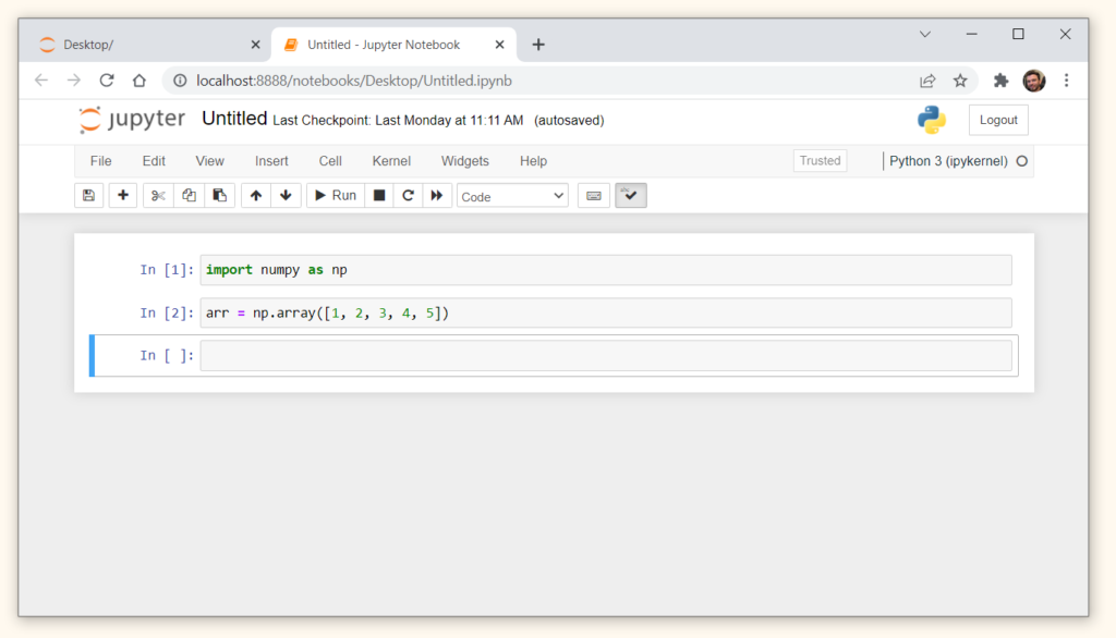
Импортируем библиотеку Numpy и создадим массив.
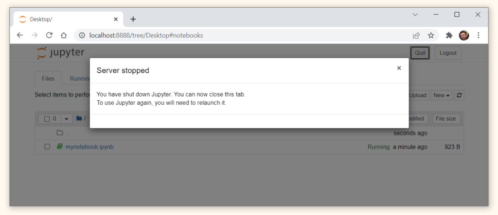
Шаг 4. Сохраните ноутбук и закройте Jupyter Notebook
Переименуйте ноутбук в mynotebook (для этого, как и в Google Colab, отредактируйте само название непосредственно в окне ноутбука). Сохранить файл можно через File → Save and Checkpoint.

Обратите внимание, помимо файла mynotebook.ipynb, Jupyter Notebook создал скрытую папку .ipynb_checkpoints. В ней хранятся файлы, которые позволяют вернуться к предыдущей сохраненной версии ноутбука (предыдущему check point). Сделать это можно, нажав File → Revert to Checkpoint и выбрав дату и время предыдущей сохраненной версии кода.
Когда вы закончили работу, закройте вкладку с ноутбуком. Остается прервать работу локального сервера, нажав Quit в правом верхнем углу.
Особенности работы
Давайте подробнее поговорим про возможности Jupyter Notebook. Снова запустим только что созданный ноутбук любым удобным способом.
Код на Python
В целом мы пишем обычный код на Питоне.
Вкладка Cell
Для управления запуском или исполнением ячеек можно использовать вкладку Cell.

Здесь мы можем, в частности:
- Запускать ячейку и оставаться в ней же через Run Cells
- Исполнять все ячейки в ноутбуке, выбрав Run All
- Исполнять все ячейки выше (Run All Above) или ниже текущей (Run All Below)
- Очистить вывод ячеек, нажав All Output → Clear
Вкладка Kernel
Командами вкладки Kernel мы управляем ядром (kernel) или вычислительным «движком» ноутбука.
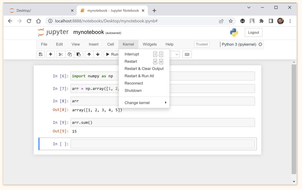
В этой вкладке мы можем, в частности:
- Прервать исполнение ячейки командой Interrupt. Это бывает полезно, если, например, исполнение кода занимает слишком много времени или в коде есть ошибка и исполнение кода не прервется самостоятельно.
- Перезапустить kernel можно командой Restart. Кроме того, можно
- очистить вывод (Restart & Clear Output) и
- заново запустить все ячейки (Restart & Run All)
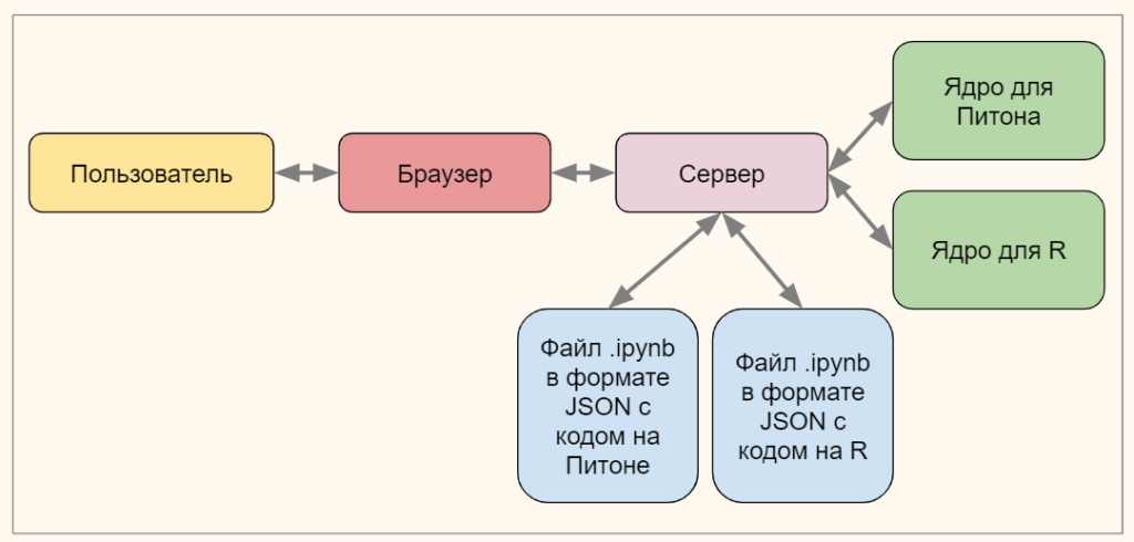
Несколько слов про то, что такое ядро и как в целом функционирует Jupyter Notebook.

Пользователь взаимодействует с ноутбуком через браузер. Браузер в свою очередь отправляет запросы на сервер. Функция сервера заключается в том, чтобы загружать ноутбук и сохранять внесенные изменения в формате JSON с расширением .ipynb. Одновременно, сервер обращается к ядру в тот момент, когда необходимо обработать код на каком-либо языке (например, на Питоне).
Такое «разделение труда» между браузером, сервером и ядром позволяет во-первых, запускать Jupyter Notebook в любой операционной системе, во-вторых, в одной программе исполнять код на нескольких языках, и в-третьих, сохранять результат в файлах одного и того же формата.
Возможность программирования на нескольких языках (а значит использование нескольких ядер) мы изучим чуть позже, а пока посмотрим как устанавливать новые пакеты для Питона внутри Jupyter Notebook.
Установка новых пакетов
Установить новые пакеты в Anaconda можно непосредственно в ячейке, введя
!pip install <package_name>. Например, попробуем установить Numpy.
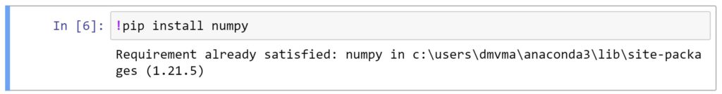
Система сообщила нам, что такой пакет уже установлен. Более того, мы видим путь к папке внутри дистрибутива Anaconda, в которой Jupyter «нашел» Numpy.
При подготовке этого занятия я использовал два компьютера, поэтому имя пользователя на скриншотах указано как user или dmvma. На вашем компьютере при указании пути к файлу используйте ваше имя пользователя.
В последующих разделах мы рассмотрим дополнительные возможности по установке пакетов через Anaconda Prompt и Anaconda Navigator.
По ссылке ниже вы можете скачать код, который мы создали в Jupyter Notebook.
Два Питона на одном компьютере
Обращу ваше внимание, что на данный момент на моем компьютере (как и у вас, если вы проделали шаги прошлого занятия) установлено два Питона, один с сайта www.python.org⧉, второй — в составе дистрибутива Anaconda.
Посмотреть на установленные на компьютеры «Питоны» можно, набрав команду
where python в Anaconda Prompt.

Указав полный или абсолютный путь (absolute path) к каждому из файлов python.exe, мы можем в интерактивном режиме исполнять код на версии 3.8 (установили с www.python.org) и на версии 3.10 (установили в составе Anaconda). При запуске файла python.exe из папки WindowsApps система предложит установить Питон из Microsoft Store.
В этом смысле нужно быть аккуратным и понимать, какой именно Питон вы используете и куда устанавливаете очередной пакет.
В нашем случае мы настроили работу так, чтобы устанавливать библиотеки для Питона с www.python.org через командную строку Windows, и устанавливать пакеты в Анаконду через Anaconda Prompt.
Убедиться в этом можно, проверив версии Питона через
python —version в обеих программах.

Теперь попробуйте ввести в них команду
pip list и сравнить установленные библиотеки.
Markdown в Jupyter Notebook
Вернемся к Jupyter Notebook. Помимо ячеек с кодом, можно использовать текстовые ячейки, в которых поддерживается язык разметки Markdown. Мы уже коротко рассмотрели этот язык на прошлом занятии, когда создавали пакет на Питоне.
По большому счету, с помощью несложных команд Markdown, вы говорите Jupyter как отформатировать ту или иную часть текста.
Рассмотрим несколько основных возможностей форматирования (для удобстства и в силу практически полного совпадения два последующих раздела приведены в ноутбуке Google Colab).
Откроем ноутбук к этому занятию⧉
Заголовки
Заголовки создаются с помощью символа решетки.
|
# Заголовок 1 ## Заголовок 2 ### Заголовок 3 #### Заголовок 4 ##### Заголовок 5 ###### Заголовок 6 |

Если перед первым символом решетки поставить знак \, Markdown просто выведет символы решетки.

Абзацы
Абзацы отделяются друг от друга пробелами.

Мы также можем разделять абзацы прямой линией.
![]()
Выделение текста
|
**Полужирный стиль** *Курсив* ~~Перечеркнутый стиль~~ |

Форматирование кода и выделенные абзацы
Мы можем выделять код внутри строки или отдельным абзацем.
|
Отформатируем код `print(‘Hello world!’)` внутри строки и отдельным абзацем «` print(‘Hello world!’) «` |

Возможно выделение и текстовых абзацев ( так называемые blockquotes).
|
> Markdown позволяет форматировать текст без использования тэгов. > > Он был создан в 2004 году Джоном Грубером и Аароном Шварцем. |

Списки
Посмотрим на создание упорядоченных и неупорядоченных списков.
|
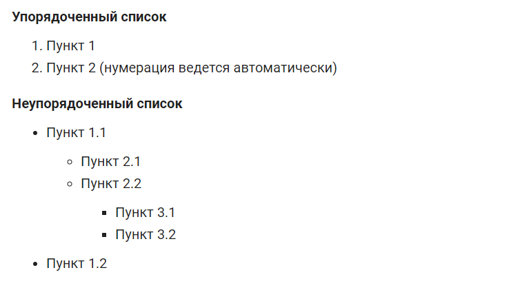
**Упорядоченный список** 1. Пункт 1 1. Пункт 2 (нумерация ведется автоматически) **Неупорядоченный список** * Пункт 1.1 * Пункт 2.1 * Пункт 2.2 * Пункт 3.1 * Пункт 3.2 * Пункт 1.2 |
Ссылки и изображения
Текст ссылки заключается в квадратные скобки, сама ссылка — в круглые.
|
[сайт проекта Jupyter](https://jupyter.org/) |
![]()
Изображение форматируется похожим образом.
|
 |
![]()
Таблицы
|
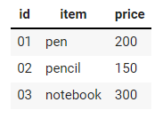
| id | item | price | |— |———-| ——| | 01 | pen | 200 | | 02 | pencil | 150 | | 03 | notebook | 300 | |
Таблицы для Markdown бывает удобно создавать с помощью специального инструмента⧉.
Формулы на LaTeX
В текстовых полях можно вставлять формулы и математические символы с помощью системы верстки, которая называется LaTeX (произносится «латэк»). Они заключаются в одинарные или двойные символы $.
Если использовать одинарный символ $, то расположенная внутри формула останется в пределах того же абзаца. Например, запись
$ y = x^2 $ даст $ y = x^2 $.
В то время как
$$ y = x^2 $$ поместит формулу в новый абзац.
$$ y = x^2 $$
Одинарный символ \ добавляет пробел. Двойной символ \\ переводит текст на новую строку.
|
$$ \hat{y} = \theta_0 + \theta_1 x_1 + \theta_2 x_2 + \ \ ... \ \ + \\ \theta_n x_n $$ |

Рассмотрим некоторые элементы синтаксиса LaTeX.
Форматирование текста
|
$ \text{just text} $ $ \textbf{bold} $ $ \textit{italic} $ $ \underline{undeline} $ |

Надстрочные и подстрочные знаки
|
hat $ \hat{x} $ bar $ \bar{x} $ vector $ \vec{x} $ tilde $ \tilde{x} $ superscript $ e^{ax + b} $ subscript $ A_{i, j} $ degree $ 90^{\circ} $ |

Скобки
Вначале рассмотрим код для скобок в пределах высоты строки.
|
$$ (a+b) \\ [a+b] \\ \{a+b\} \\ \langle x+y \rangle \\ |x+y| \\ \|x+y\| $$ |

Кроме того, с помощью
\left(,
\right), а также
\left[,
\right] и так далее можно увеличить высоту скобки. Сравните.
|
$$ \left(\frac{1}{2}\right) \qquad (\frac{1}{2}) $$ |

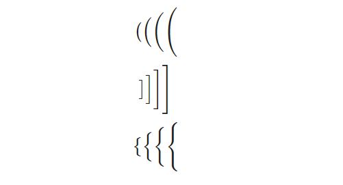
Также можно использовать отдельные команды для скобок различного размера.
|
$$ \big( \Big( \bigg( \Bigg( \\ \big] \Big] \bigg] \Bigg] \\ \big\{ \Big\{ \bigg\{ \Bigg\{ $$ |
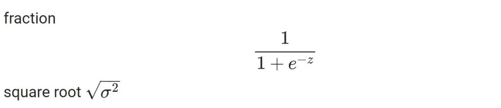
Дробь и квадратный корень
|
fraction $$ \frac{1}{1+e^{—z}} $$ square root $ \sqrt{\sigma^2} $ |
Греческие буквы
|
1 2 3 4 5 6 7 8 9 10 11 12 13 14 15 16 17 18 19 20 21 22 23 24 25 26 27 28 29 30 31 32 |
|Uppercase | LaTeX |Lowercase | LaTeX | RU | |————— |———— |————— |———— |———— | |————— |———— |$\alpha$ |\\alpha | альфа | |————— |———— |$\beta$ |\\beta | бета | |$\Gamma$ |\\Gamma |$\gamma$ |\\gamma | гамма | |$\Delta$ |\\Delta |$\delta$ |\\delta | дельта | |————— |———— |$\epsilon$ |\\epsilon | эпсилон | |————— |———— |$\varepsilon$ |\\varepsilon | ———— | |————— |———— |$\zeta$ |\\zeta | дзета | |————— |———— |$\eta$ |\\eta | эта | |$\Theta$ |\\Theta |$\theta$ |\\theta | тета | |————— |———— |$\vartheta$ |\\vartheta | ———— | |————— |———— |$\iota$ |\\iota | йота | |————— |———— |$\kappa$ |\\kappa | каппа | |$\Lambda$ |\\Lambda |$\lambda$ |\\lambda | лямбда | |————— |———— |$\mu$ |\\mu | мю | |————— |———— |$\nu$ |\\nu | ню | |$\Xi$ |\\Xi |$\xi$ |\\xi | кси | |————— |———— |$\omicron$ |\\omicron | омикрон | |$\Pi$ |\\Pi |$\pi$ |\\pi | пи | |————— |———— |$\varpi$ |\\varpi | ———— | |————— |———— |$\rho$ |\\rho | ро | |————— |———— |$\varrho$ |\\varrho | ———— | |$\Sigma$ |\\Sigma |$\sigma$ |\\sigma | сигма | |————— |———— |$\varsigma$ |\\varsigma | ———— | |————— |———— |$\tau$ |\\tau | тау | |$\Upsilon$ |\\Upsilon |$\upsilon$ |\\upsilon | ипсилон | |$\Phi$ |\\Phi |$\phi$ |\\phi | фи | |————— |———— |$\varphi$ |\\varphi | ———— | |————— |———— |$\chi$ |\\chi | хи | |$\Psi$ |\\Psi |$\psi$ |\\psi | пси | |$\Omega$ |\\Omega |$\omega$ |\\omega | омега | |


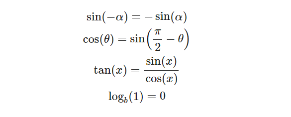
Латинские обозначения
|
$$ \sin(—\alpha) = —\sin(\alpha) \\ \cos(\theta)=\sin \left( \frac{\pi}{2}—\theta \right) \\ \tan(x) = \frac{\sin(x)}{\cos(x)} \\ \log_b(1) = 0 \\ $$ |
Логические символы и символы множества
|
1 2 3 4 5 6 7 8 9 10 11 12 13 14 15 16 17 18 19 |
| LaTeX | symbol | | ——————————— | ————————————— | |\Rightarrow | $ \Rightarrow $ | |\rightarrow | $ \rightarrow $ | |\longleftrightarrow | $ \Leftrightarrow $ | |\cap | $ \cap $ | |\cup | $ \cup $ | |\subset | $ \subset $ | |\in | $ \in $ | |\notin | $ \notin $ | |\varnothing | $ \varnothing $ | |\neg | $ \neg $ | |\forall | $ \forall $ | |\exists | $ \exists $ | |\mathbb{N} | $ \mathbb{N} $ | |\mathbb{Z} | $ \mathbb{Z} $ | |\mathbb{Q} | $ \mathbb{Q} $ | |\mathbb{R} | $ \mathbb{R} $ | |\mathbb{C} | $ \mathbb{C} $ | |

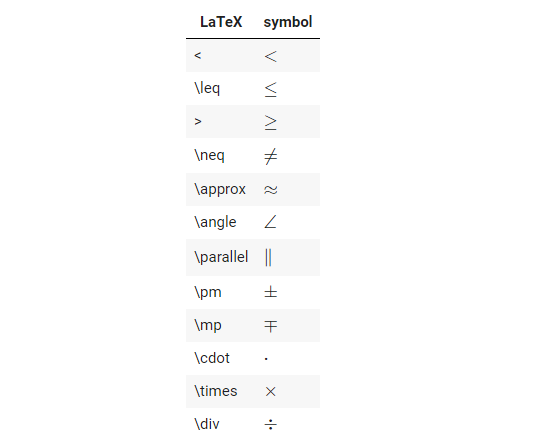
Другие символы
|
| LaTeX | symbol | | ——————————— | ————————————— | | < | $ < $ | | \leq | $ \leq $ | | > | $ \geq $ | | \neq | $ \neq $ | | \approx | $ \approx $ | | \angle | $ \angle $ | | \parallel | $ \parallel $ | | \pm | $ \pm $ | | \mp | $ \mp $ | | \cdot | $ \cdot $ | | \times | $ \times $ | | \div | $ \div $ | |
Кусочная функция и система уравнений
Посмотрим на запись функции sgn (sign function) средствами LaTeX.
|
$$ sgn(x) = \left\{ \begin{array}\\ 1 & \mbox{if } \ x \in \mathbf{N}^* \\ 0 & \mbox{if } \ x = 0 \\ —1 & \mbox{else.} \end{array} \right. $$ |

Схожим образом записывается система линейных уравнений.
|
$$ \left\{ \begin{matrix} 4x + 3y = 20 \\ —5x + 9y = 26 \end{matrix} \right. $$ |

Горизонтальная фигурная скобка
|
$$ \overbrace{ \underbrace{a}_{real} + \underbrace{b}_{imaginary} i} ^{\textit{complex number}} $$ |

Предел, производная, интеграл
|
1 2 3 4 5 6 7 8 9 10 11 12 13 14 15 16 17 18 19 20 21 22 23 24 25 26 27 28 |
Пределы: $$ \lim_{x \to +\infty} f(x) $$ $$ \lim_{x \to —\infty} f(x) $$ $$ \lim_{x \to с} f(x) $$ Производная (нотация Лагранжа): $$ f‘(x) $$ Частная производная (нотация Лейбница): $$ \frac{\partial f}{\partial x} $$ Градиент: $$ \nabla f(x_1, x_2) = \begin{bmatrix} \frac{\partial f}{\partial x_1} \\ \frac{\partial f}{\partial x_2} \end{bmatrix} $$ Интеграл: $$\int_{a}^b f(x)dx$$ |

Сумма и произведение
|
Сумма: $$ \sum\limits_{i=1}^n a_{i} $$ $$\sum_{i=1}^n a_{i} $$ Произведение: $$\prod_{j=1}^m a_{j}$$ |

Матрица
|
1 2 3 4 5 6 7 8 9 10 11 12 13 14 15 16 17 18 19 20 21 22 23 24 25 26 27 28 29 30 31 32 33 34 35 36 37 38 39 40 41 42 43 44 45 46 47 48 49 50 51 52 53 |
Без скобок (plain): $$ \begin{matrix} 1 & 2 & 3\\ a & b & c \end{matrix} $$ Круглые скобки (parentheses, round brackets): $$ \begin{pmatrix} 1 & 2 & 3\\ a & b & c \end{pmatrix} $$ Квадратные скобки (square brackets): $$ \begin{bmatrix} 1 & 2 & 3\\ a & b & c \end{bmatrix} $$ Фигурные скобки (curly brackets, braces): $$ \begin{Bmatrix} 1 & 2 & 3\\ a & b & c \end{Bmatrix} $$ Прямые скобки (pipes): $$ \begin{vmatrix} 1 & 2 & 3\\ a & b & c \end{vmatrix} $$ Двойные прямые скобки (double pipes): $$ \begin{Vmatrix} 1 & 2 & 3\\ a & b & c \end{Vmatrix} $$ |

Программирование на R
Jupyter Notebook позволяет писать код на других языках программирования, не только на Питоне. Попробуем написать и исполнить код на R, языке, который специально разрабатывался для data science.
Вначале нам понадобится установить kernel для R. Откроем Anaconda Prompt и введем следующую команду
conda install -c r r-irkernel. В процессе установки система спросит продолжать или нет (Proceed ([y]/n)?). Нажмите y + Enter.
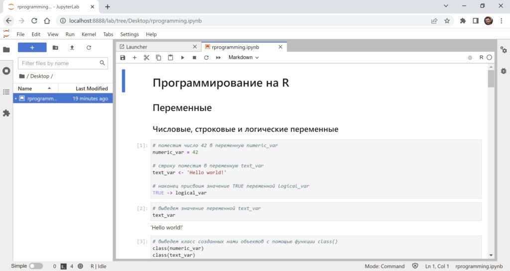
Откройте Jupyter Notebook. В списке файлов создайте ноутбук на R. Назовем его rprogramming.

После установки нового ядра и создания еще одного файла .ipynb схема работы нашего Jupyter Notebook немного изменилась.
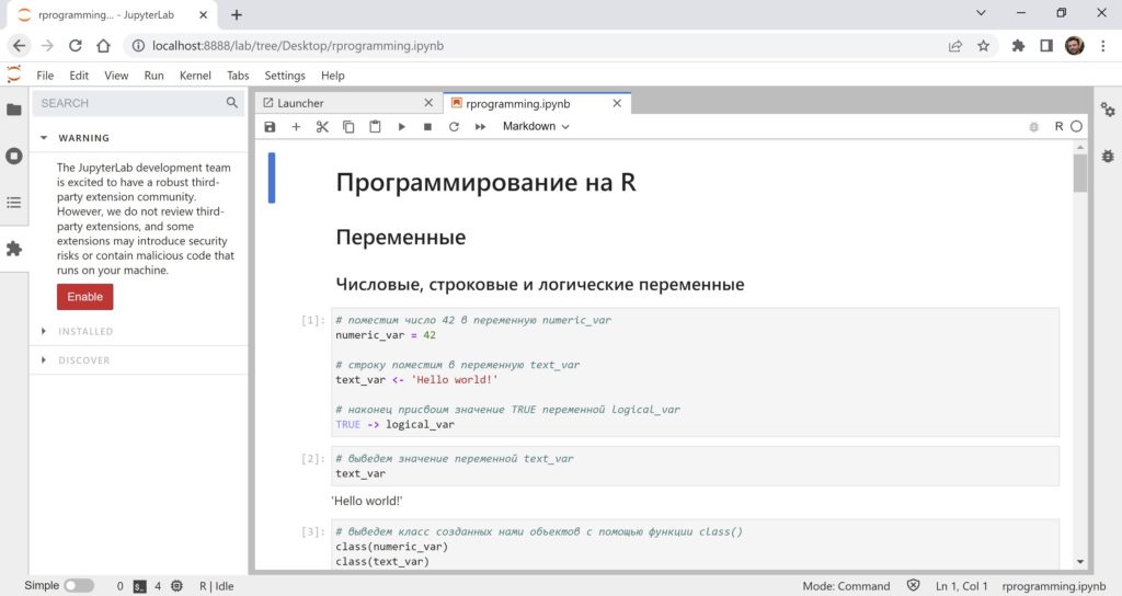
Теперь мы готовы писать код на R. Мы уже начали знакомиться с этим языком, когда изучали парадигмы программирования. Сегодня мы рассмотрим основные типы данных и особенности синтаксиса.
Переменные в R
Числовые, строковые и логические переменные
Как и в Питоне, в R мы можем создавать числовые (numeric), строковые (character) и логические (logical) переменные.
|
# поместим число 42 в переменную numeric_var numeric_var = 42 # строку поместим в переменную text_var text_var <— ‘Hello world!’ # наконец присвоим значение TRUE переменной logical_var TRUE -> logical_var |
Для присвоения значений можно использовать как оператор
=, так и операторы присваивания
<— и
->. Обратите внимание, используя
-> мы можем поместить значение слева, а переменную справа.
Посмотрим на результат (в Jupyter Notebook можно обойтись без функции print()).
Выведем класс созданных нами объектов с помощью функции class().
|
class(numeric_var) class(text_var) class(logical_var) |
|
‘numeric’ ‘character’ ‘logical’ |
Тип данных можно посмотреть с помощью функции typeof().
|
typeof(numeric_var) typeof(text_var) typeof(logical_var) |
|
‘double’ ‘character’ ‘logical’ |
Хотя вывод этих функций очень похож, мы, тем не менее, видим, что классу numeric соответствует тип данных double (число с плавающей точкой с двумя знаками после запятой).
Числовые переменные: numeric, double, integer
По умолчанию, в R и целые числа, и дроби хранятся в формате double.
|
# еще раз поместим число 42 в переменную numeric_var numeric_var <— 42 # выведем тип данных typeof(numeric_var) |
Принудительно перевести 42 в целочисленное значение можно с помощью функции as.integer().
|
int_var <— as.integer(numeric_var) typeof(int_var) |
Кроме того, если после числа поставить L, это число автоматически превратится в integer.
Превратить integer обратно в double можно с помощью функций as.double() и as.numeric().
|
typeof(as.double(int_var)) typeof(as.numeric(42L)) |
Если число хранится в формате строки, его можно перевести обратно в число (integer или double).
|
text_var <— ’42’ typeof(text_var) |
|
typeof(as.numeric(text_var)) # можно также использовать as.double() typeof(as.integer(text_var)) |
Вектор
Вектор (vector) — это одномерная структура, которая может содержать множество элементов одного типа. Вектор можно создать с помощью функции c().
|
# создадим вектор с информацией о продажах товара в магазине за неделю (в тыс. рублей) sales <— c(24, 28, 32, 25, 30, 31, 29) sales |
С помощью функций length() и typeof() мы можем посмотреть соответственно общее количество элементов и тип данных каждого из них.
|
# посмотрим на общее количество элементов и тип данных каждого из них length(sales) typeof(sales) |
У вектора есть индекс, который (в отличие, например, от списков в Питоне), начинается с единицы.
При указании диапазона выводятся и первый, и последний его элементы.
Отрицательный индекс убирает элементы из вектора.
Именованный вектор (named vector) создается с помощью функции names().
|
# создадим еще один вектор с названиями дней недели days_vector <— c(‘Понедельник’, ‘Вторник’, ‘Среда’, ‘Четверг’, ‘Пятница’, ‘Суббота’, ‘Воскресенье’) days_vector |
|
‘Понедельник’ ‘Вторник’ ‘Среда’ ‘Четверг’ ‘Пятница’ ‘Суббота’ ‘Воскресенье’ |
|
# создадим именованный вектор с помощью функции names() names(sales) <— days_vector sales |

Выводить элементы именованного вектора можно не только по числовому индексу, но и по их названиям.
Список
В отличие от вектора, список (list) может содержать множество элементов различных типов.
|
# список создается с помощью функции list() list(‘DS’, ‘ML’, c(21, 24), c(TRUE, FALSE), 42.0) |
|
[[1]] [1] «DS» [[2]] [1] «ML» [[3]] [1] 21 24 [[4]] [1] TRUE FALSE [[5]] [1] 42 |
Матрица
Матрица (matrix) в R — это двумерная структура, содержащая одинаковый тип данных (чаще всего числовой). Матрица создается с помощью функции matrix() с параметрами data, nrow, ncol и byrow.
- data — данные для создания матрицы
- nrow и ncol — количество строк и столбцов
- byrow — параметр, указывающий заполнять ли элементы матрицы построчно (TRUE) или по столбцам (FALSE)
Рассмотрим несколько примеров. Cоздадим последовательность целых чисел (по сути, тоже вектор).
|
# для этого подойдет функция seq() sqn <— seq(1:9) sqn typeof(sqn) |
|
1 2 3 4 5 6 7 8 9 ‘integer’ |
Используем эту последовательность для создания двух матриц.
|
# создадим матрицу, заполняя значения построчно mtx <— matrix(sqn, nrow = 3, ncol = 3, byrow = TRUE) mtx |

|
# теперь создадим матрицу, заполняя значения по столбцам mtx <— matrix(sqn, nrow = 3, ncol = 3, byrow = FALSE) mtx |

Зададим названия для строк и столбцов второй матрицы.
|
# создадим два вектора с названиями строк и столбцов rows <— c(‘Row 1’, ‘Row 2’, ‘Row 3’) cols <— c(‘Col 1’, ‘Col 2’, ‘Col 3’) # используем функции rownames() и colnames(), # чтобы передать эти названия нашей матрице rownames(mtx) <— rows colnames(mtx) <— cols # посмотрим на результат mtx |
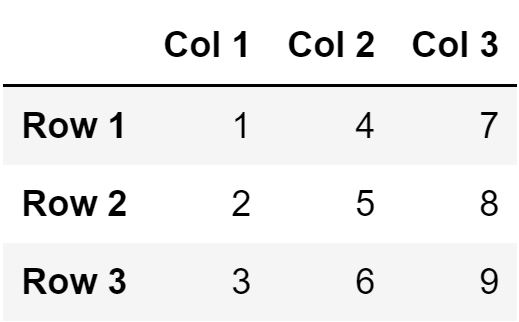
Посмотрим на размерность этой матрицы с помощью функции dim().
Массив
В отличие от матрицы, массив (array) — это многомерная структура. Создадим трехмерный массив размерностью 3 х 2 х 3. Вначале создадим три матрицы размером 3 х 2.
|
# создадим три матрицы размером 3 х 2, # заполненные пятерками, шестерками и семерками a <— matrix(5, 3, 2) b <— matrix(6, 3, 2) c <— matrix(7, 3, 2) |
Теперь соединим их с помощью функции array(). Передадим этой функции два параметра в форме векторов: данные (data) и размерность (dim).
|
arr <— array(data = c(a, b, c), # вектор с матрицами dim = c(3, 2, 3)) # вектор размерности print(arr) |
|
1 2 3 4 5 6 7 8 9 10 11 12 13 14 15 16 17 18 19 20 |
, , 1 [,1] [,2] [1,] 5 5 [2,] 5 5 [3,] 5 5 , , 2 [,1] [,2] [1,] 6 6 [2,] 6 6 [3,] 6 6 , , 3 [,1] [,2] [1,] 7 7 [2,] 7 7 [3,] 7 7 |
Факторная переменная
Факторная переменная или фактор (factor) — специальная структура для хранения категориальных данных. Вначале немного теории.
Как мы узнаем на курсе анализа данных, категориальные данные бывают номинальными и порядковыми. Номинальные категориальные (nominal categorical) данные представлены категориями, в которых нет естественного внутреннего порядка. Например, пол или цвет волос человека, марка автомобиля могут быть отнесены к определенным категориям, но не могут быть упорядочены.
Порядковые категориальные (ordinal categorical) данные наоборот обладают внутренним, свойственным им порядком. К таким данным относятся шкала удовлетворенности потребителей, класс железнодорожного билета, должность или звание, а также любая количественная переменная, разбитая на категории (например, низкий, средний и высокий уровень зарплат).
Посмотрим, как учесть такие данные с помощью R. Начнем с номинальных данных.
|
# предположим, что мы собрали данные о цветах нескольких автомобилей и поместили их в вектор color_vector <— c(‘blue’, ‘blue’, ‘white’, ‘black’, ‘yellow’, ‘white’, ‘white’) # преобразуем этот вектор в фактор с помощью функции factor() factor_color <— factor(color_vector) factor_color |

Как вы видите, функция factor() разбила данные на категории, при этом эти категории остались неупорядоченными. Посмотрим на класс созданного объекта.
Теперь поработаем с порядковыми данными.
|
# возьмем данные измерений температуры, выраженные категориями temperature_vector <— c(‘High’, ‘Low’, ‘High’,‘Low’, ‘Medium’, ‘High’, ‘Low’) # создадим фактор factor_temperature <— factor(temperature_vector, # указав параметр order = TRUE order = TRUE, # а также вектор упорядоченных категорий levels = c(‘Low’, ‘Medium’, ‘High’)) # посмотрим на результат factor_temperature |

Выведем класс созданного объекта.
|
class(factor_temperature) |
Добавлю, что количество элементов в каждой из категорий можно посмотреть с помощью функции summary().
|
summary(factor_temperature) |

Датафрейм
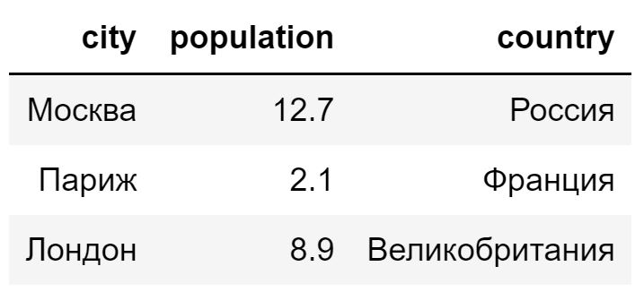
Датафрейм в R выполняет примерно ту же функцию, что и в Питоне. С помощью функции data.frame() создадим простой датафрейм, гда параметрами будут названия столбцов, а аргументами — векторы их значений.
|
df <— data.frame(city = c(‘Москва’, ‘Париж’, ‘Лондон’), population = c(12.7, 2.1, 8.9), country = c(‘Россия’, ‘Франция’, ‘Великобритания’)) df |
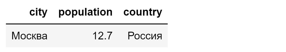
Доступ к элементам датафрейма можно получить по индексам строк и столбцов, которые также начинаются с единицы.
|
# выведем значения первой строки и первого столбца df[1, 1] |

|
# выведем всю первую строку df[1,] |
|
# выведем второй столбец df[,2] |
Получить доступ к столбцам можно и так.
Дополнительные пакеты
Как и в Питоне, в R мы можем установить дополнительные пакеты через Anaconda Prompt. Например, установим пакет ggplot2 для визуализации данных. Для этого введем команду
conda install r-ggplot2.
В целом команда установки пакетов для R следующая:
conda install r-<package_name>.
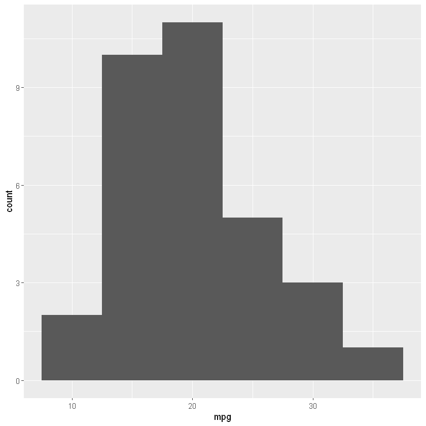
Продемонстрируем работу с этим пакетом с помощью несложного датасета mtcars.
|
# импортируем библиотеку datasets library(datasets) # загрузим датасет mtcars data(mtcars) # выведем его на экран mtcars |

Теперь импортируем установленную ранее библиотеку ggplot2.
Построим гистограмму по столбцу mpg (miles per galon, расход в милях на галлон топлива). Для построения гистограммы нам потребуется через «+» объединить две функции:
- функцию ggplot(), которой мы передадим наши данные и еще одну функцию aes(), от англ. aesthetics, которая свяжет ось x нашего графика и столбец данных mpg, а также
- функцию geom_histogram() с параметрами bins (количество интервалов) и binwidth (их ширина), которая и будет отвечать за создание гистограммы
|
# данными будет датасет mtcars, столбцом по оси x — mpg ggplot(data = mtcars, aes(x = mpg)) + # типом графика будет гистограмма с 10 интервалами шириной 5 миль на галлон каждый geom_histogram(bins = 10, binwidth = 5) |
Примерно также мы можем построить график плотности распределения (density plot). Только теперь мы передадим функции aes() еще один параметр
fill = as.factor(vs), который (предварительно превратив столбец в фактор через as.factor()) позволит разбить данные на две категории по столбцу vs. В этом датасете признак vs указывает на конфигурацию двигателя (расположение цилиндров), v-образное, v-shaped (vs == 0) или рядное, straight (vs == 1).
Кроме того, для непосредственного построения графика мы будем использовать новую функцию geom_density() с параметром alpha, отвечающим за прозрачность заполнения пространства под кривыми.
|
ggplot(data = mtcars, aes(x = mpg, fill = as.factor(vs))) + geom_density(alpha = 0.3) |

Дополнительно замечу, что к столбцам датафрейма можно применять множество различных функций, например, рассчитать среднее арифметическое или медиану с помощью несложных для запоминания mean() и median().
|
mean(mtcars$mpg) median(mtcars$mpg) |
Кроме того, мы можем применить уже знакомую нам функцию summary(), которая для количественного столбца выдаст минимальное и максимальное значения, первый (Q1) и третий (Q2) квартили, а также медиану и среднее значение.
|
Min. 1st Qu. Median Mean 3rd Qu. Max. 10.40 15.43 19.20 20.09 22.80 33.90 |
В файле ниже содержится созданный нами код на R.
Вернемся к основной теме занятия.
Подробнее про Anaconda
Conda
Программа conda, как уже было сказано, объединяет в себе систему управления пакетами (как pip) и, кроме того, позволяет создавать окружения.
Идея виртуального окружения (virtual environment) заключается в том, что если в рамках вашего проекта вы, например, используете определенную версию библиотеки Numpy и установка более ранней или более поздней версии приведет к сбоям в работе вашего кода, хорошим решением была бы изоляция нужной версии Numpy, а также всех остальных используемых вами библиотек. Именно для этого и нужно виртуальное окружение.
Рассмотрим, как мы можем устанавливать пакеты и создавать окружения через Anaconda Prompt и через Anaconda Navigator.
Anaconda Prompt
Про пакеты. По аналогии с pip, установленные (в текущем окружении) пакеты можно посмотреть с помощью команды
conda list.
Установить пакет можно с помощью команды
conda install <package_name>. Обновить пакет можно через
conda update <package_name>. Например, снова попробуем установить Numpy. о

Про окружения. По умолчанию мы работаем в базовом окружении (base environment). Посмотреть, какие в целом установлены окружения можно с помощью команды
conda info —envs.

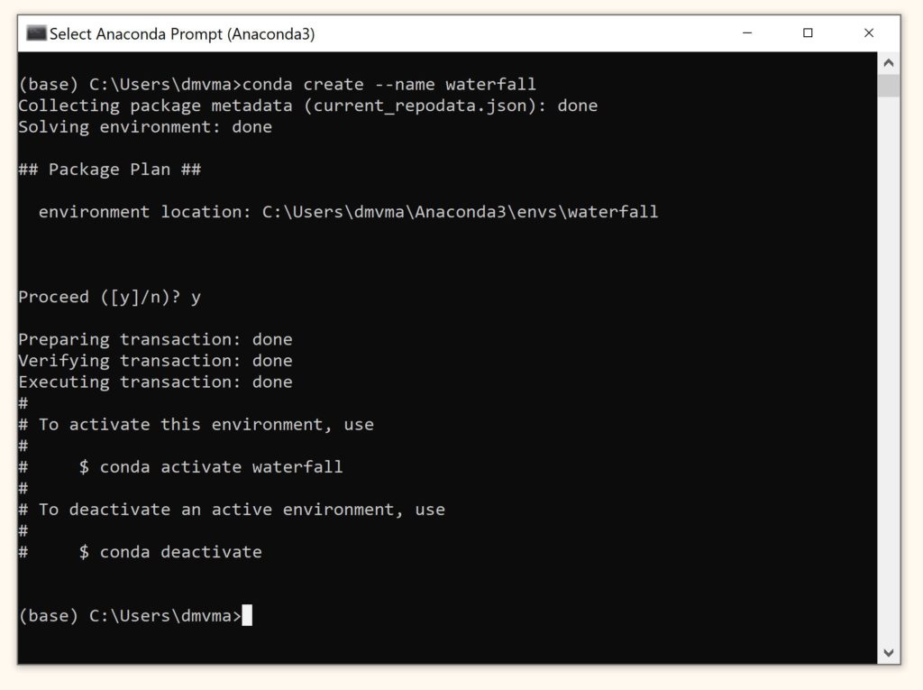
Как вы видите, пока у нас есть только одно окружение. Давайте создадим еще одно виртуальное окружение и назовем его, например, waterfall.
Введите команду
conda create —name waterfall.
Введем две команды
- conda activate waterfall для активации нового окружения
- conda list для того, чтобы посмотреть установленные в нем пакеты

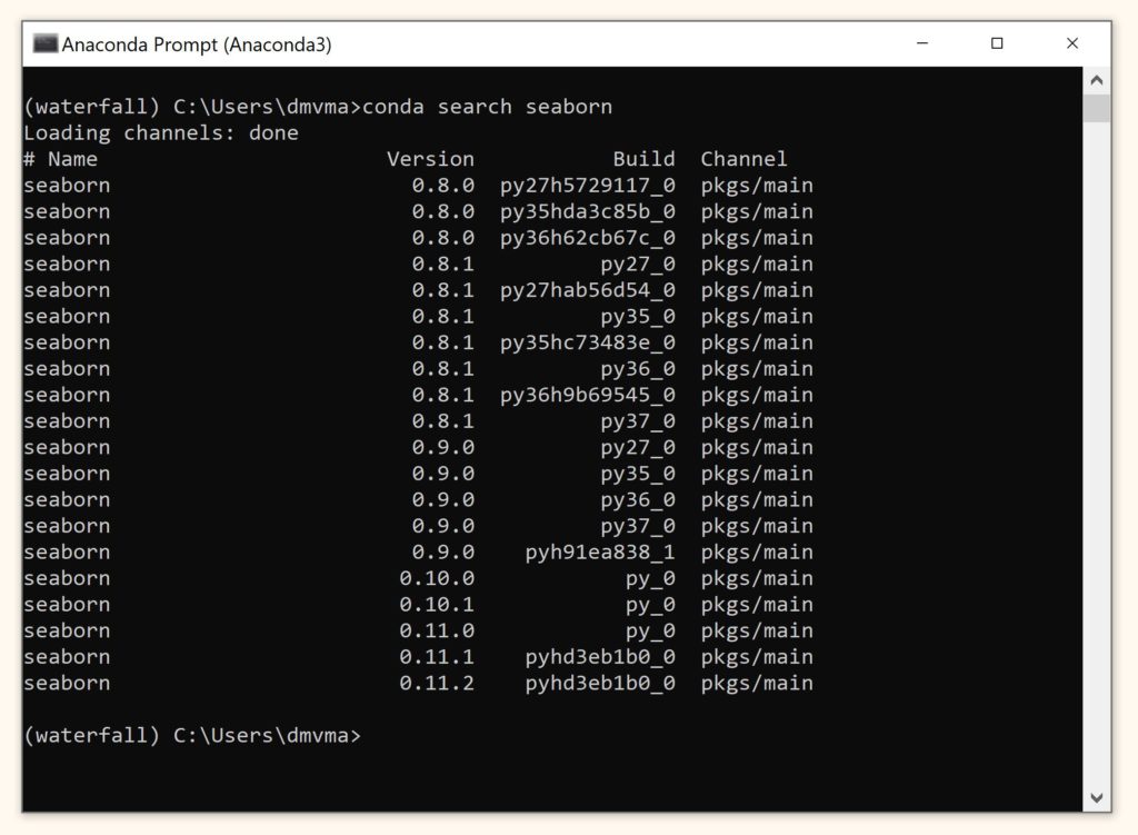
Как вы видите, в новом окружении нет ни одного пакета. Введем
conda search seaborn, чтобы посмотреть какие версии этого пакета доступны для скачивания.
Скачаем этот пакет через
conda install seaborn. Проверим установку с помощью
conda list.
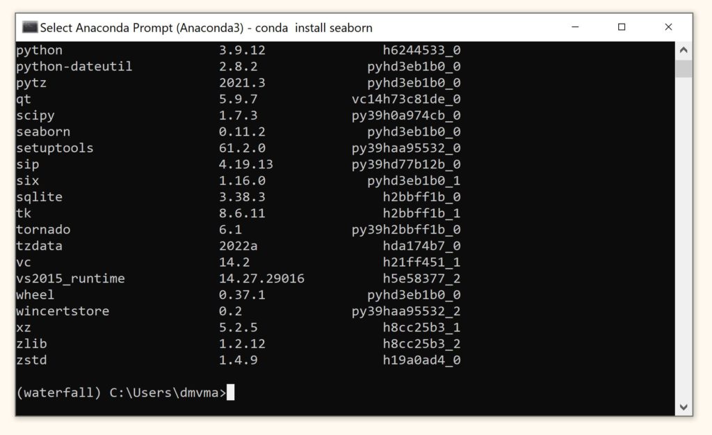
Как вы видите, помимо seaborn было установлено множество других необходимых для работы пакета библиотек. Вернуться в базовое окружение можно с помощью команд
conda activate base или
conda deactivate.
Импорт модулей и переменная path
На прошлом занятии мы научились импортировать собственный модуль в командной строке Windows (cmd).
Посмотрим, отличается ли содержимое списка path для двух установленных версий Питона. Для этого в командной строке Windows и в Anaconda Prompt перейдем в интерактивный режим с помощью
python. Затем введем

Как мы видим, пути в переменной path будут отличаться и это нужно учитывать, если мы хотим локально запускать собственные модули.
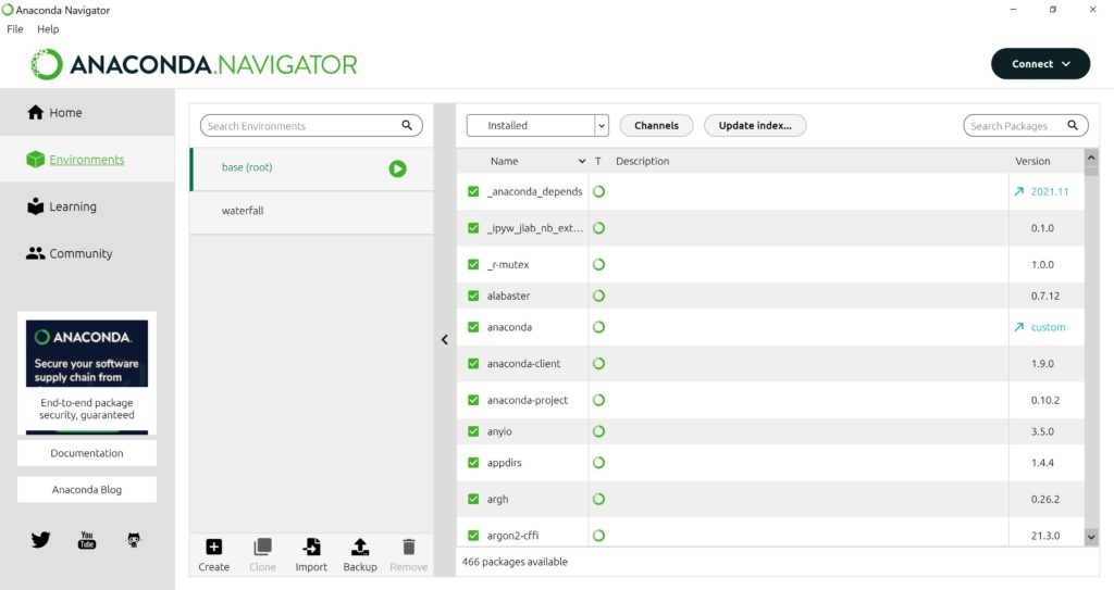
Anaconda Navigator
Запускать программы, управлять окружениями и устанавливать необходимые библиотеки можно также через Anaconda Nagivator. На вкладке Home вы видите программы, которые можно открыть (launch) или установить (install) для текущего окружения.

На вкладке Environments отображаются созданные нами окружения (в частности, окружение waterfall, которое мы создали ранее) и содержащиеся в них пакеты.
В целом интерфейс интуитивно понятен, и так как мы уже познакомились с принципом создания окружений и установки в них дополнительных пакетов, уверен, работа с Anaconda Navigator сложностей не вызовет.
Прежде чем завершить, обратимся к еще одной программе для интерактивного программирования JupyterLab.
JupyterLab
JupyterLab — расширенная версия Jupyter Notebook, которая также входит в дистрибутив Anaconda. Запустить эту программу можно через Anaconda Navigator или введя команду
jupyter lab в Anaconda Prompt.
После запуска вы увидите вкладку Launcher, в которой можно создать новый ноутбук (Notebook) на Питоне или R, открыть консоль (Console) на этих языках, а также создать файлы в различных форматах (Other). Слева вы видите список папок компьютера.
В разделе Console нажмем на Python 3 (ipykernel). Введем несложный код (см. ниже) и исполним его, нажимая Shift + Enter.
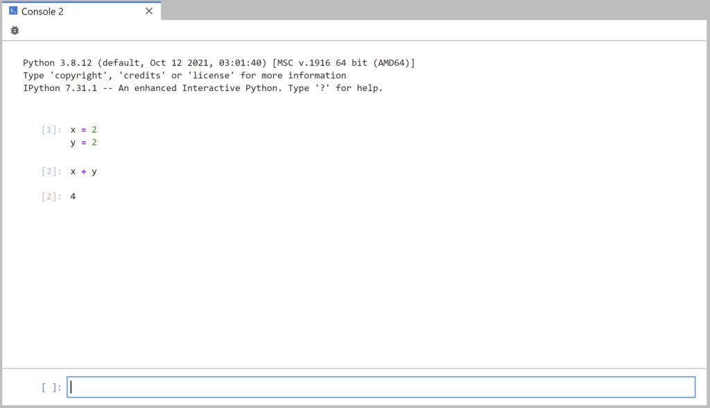
Как вы видите, здесь мы можем писать код на Питоне так же, как мы это делали в командной строке Windows на прошлом занятии. Закроем консоль.
В файловой системе слева мы можем открывать уже созданные ноутбуки. Например, откроем ноутбук на R rprogramming.ipynb.
В левом меню на второй сверху вкладке мы видим открытые горизонтальные вкладки (Launcher и rprogramming.ipynb), а также запущенные ядра (kernels).
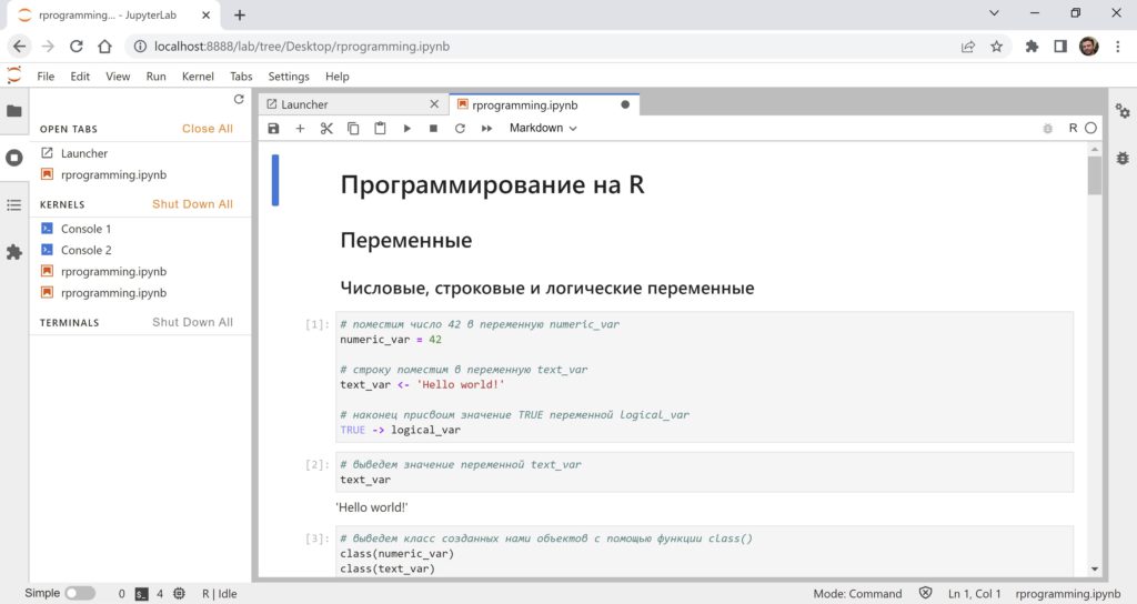
Консольные ядра (Console 1 и Console 2) можно открыть (по сути, мы снова запустим консоль).

Две оставшиеся вертикальные вкладки открывают доступ к автоматическому оглавлению (content) и расширениям (extensions).

Вкладки Run и Kernel в верхнем меню JupyterLab в целом аналогичны вкладкам Cell и Kernel в JupyterNotebook.
Подведем итог
На сегодняшнем занятии мы познакомились с программой Jupyter Notebook, а также изучили дистрибутив Anaconda, в состав которого входит эта программа.
Говоря о программе Jupyter Notebook, мы узнали про возможности работы с ячейками и ядром программы. Кроме того, мы познакомились с языком разметки Markdown и написанием формул с помощью языка верстки LaTeX.
После этого мы установили ядро для программирования на R и рассмотрели основы этого языка.
При изучении дистрибутива Anaconda мы позникомились с системой conda и попрактиковались в установке библиотек и создании окружений через Anaconda Prompt и Anaconda Navigator.
Наконец мы узнали про особенности программы JupyterLab.
Вопросы для закрепления
Вопрос. Что такое Anaconda?
Посмотреть правильный ответ
Ответ: Anaconda — это дистрибутив Питона (с репозиторием пакетов) и отдельной программой управления окружениями и пакетами conda. Пользователь может взаимодействовать с этой программой через терминал (Anaconda Prompt) и графический интерфейс (Anaconda Navigator).
Помимо этого, в дистрибутив Anaconda входят, среди прочих, программы Jupyter Notebook и JupyterLab.
Вопрос. Какой тип ячеек доступен в Jupyter Notebook?
Посмотреть правильный ответ
Ответ: в Jupyter Notebook есть два основных типа ячеек — ячейки для написания кода (в частности, на Питоне и R) и текстовые ячейки, поддерживающие Markdown и LaTeX.
Вопрос. Для чего нужно виртуальное окружение?
Посмотреть правильный ответ
Ответ: виртуальное окружение (virtual environment) позволяет установить и изолировать определенные версии Питона и его пакетов. Таким образом код, написанный с учетом конкретной версии Питона и дополнительных библиотек, исполнится без ошибок.
Ответы на вопросы
Вопрос. Можно ли исполнить код на R в Google Colab?
Ответ. Да, это возможно. Причем двумя способами.
Способ 1. Откройте ноутбук. Введите и исполните команду
%load_ext rpy2.ipython. В последующих ячейках введите
%R, чтобы в этой же строке написать код на R или
%%R, если хотите, чтобы вся ячейка исполнилась как код на R (так называемые магические команды).
В этом случае мы можем исполнять код на двух языках внутри одного ноутбука.
|
# введем магическую команду, которая позволит программировать на R %load_ext rpy2.ipython |
|
# команда %%R позволит Colab распознать ячейку как код на R %%R # кстати, числовой вектор можно создать просто с помощью двоеточия x <— 1:10 x |
|
# при этом ничто не мешает нам продолжать писать код на Питоне import numpy as np np.mean([1, 2, 3]) |
Приведенный выше код можно найти в дополнительных материалах⧉ к занятию.
Способ 2. Если вы хотите, чтобы весь код исполнялся на R (как мы это делали в Jupyter Notebook), создайте новый ноутбук используя одну из ссылок ниже:
- https://colab.research.google.com/#create=true&language=r⧉
- https://colab.to/r⧉
Теперь, если вы зайдете на вкладку Runtime → Change runtime type, то увидите, что можете выбирать между Python и R.

Выведем версию R в Google Colab.
|
‘R version 4.2.0 (2022-04-22)’ |
Посмотреть на установленные пакеты можно с помощью
installed.packages(). Созданный ноутбук Google Colab на R доступен по ссылке⧉.
Вопрос. Очень медленно загружается Anaconda. Можно ли что-то сделать?
Ответ. Можно работать через Anaconda Prompt, эта программа быстрее графического интерфейса Anaconda Navigator.
Кроме того, можно использовать дистрибутив Miniconda⧉, в который входит conda, Питон и несколько ключевых пакетов. Остальные пакеты устанавливаются вручную по мере необходимости.
Вопрос. Разве Jupyter не должен писаться через i, как Jupiter?
Ответ. Вы правы в том плане, что название Jupyter Notebook происходит не от планеты Юпитер, которая по-английски как раз пишется через i (Jupiter), а представляет собой акроним от названий языков программирования Julia, Python и R.
При этом, как утверждают разработчики⧉, слово Jupyter также отсылает к тетрадям (notebooks) Галилея, в которых он, в частности, документировал наблюдение за лунами Юпитера.
Вопрос. В каких еще программах можно писать код на Питоне и R?
Ответ. Таких программ несколько. Довольно удобно пользоваться облачным решением Kaggle. Там можно создавать как скрипты (scripts, в том числе RMarkdown Scripts), так и ноутбуки на Питоне и R. Подробнее можно почитать в документации⧉ на их сайте.
Вопрос. Можно ли создать виртуальное окружение каким-либо другим способом помимо программы conda?
Ответ. Да, можно. Вот здесь⧉ есть хорошая видео-инструкция.
Вот коротко какие шаги нужно выполнить.
Вначале убедитесь, что у вас уже установлен Питон. В нем по умолчанию содержится модуль venv, который как раз предназначен для создания виртуального окружения.
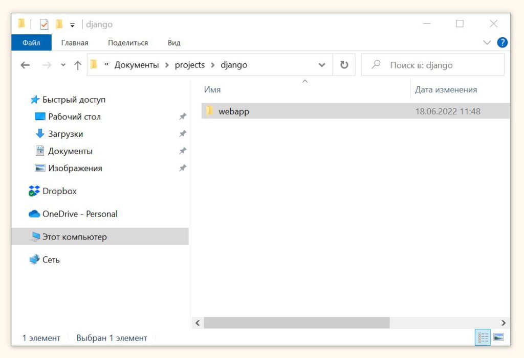
Шаг 1. Создайте папку с вашим проектом, например, пусть это будет папка webapp для веб-приложения на популярном фреймворке для Питона Django.
Шаг 2. В командной строке перейдите в папку webapp.
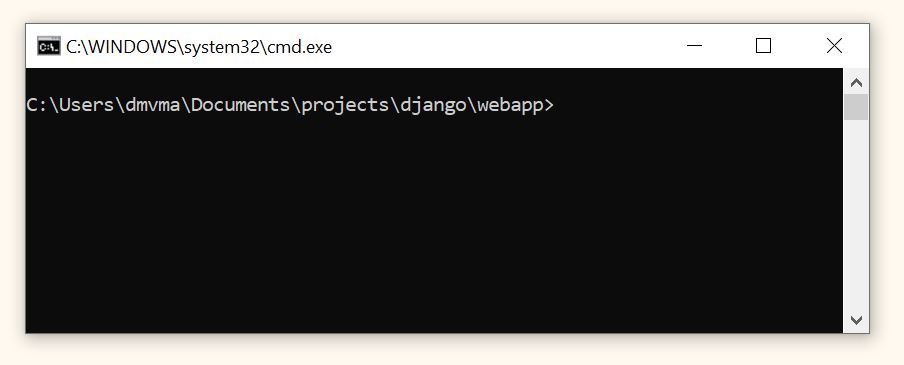
Затем введите команду для создания виртуального окружения.
По сути мы говорим Питону создать окружение djenv (название может быть любым) с помощью модуля venv. Переключатель (flag или switch)
-m подсказывает питону, что venv — это модуль, а не файл.
После выполнения этой команды создается папка djenv виртуального окружения.

Шаг 3. Активируем это виртуальное окружение следующей командой.

Здесь мы обращаемся к файлу activate внутри папки Scripts. Как вы видите, название окружения появилось слева от пути к папке.
Теперь через pip можно устанавливать пакеты, которые будут «видны» только внутри виртуального окружения djenv.
Шаг 4. Выйти из этого виртуального окружения можно с помощью команды deactivate. Если вам нужно удалить окружение, сначала деактивируйте его, а затем вручную удалите соответствующую папку.
На следующем занятии мы поговорим про такую важную тему, как регулярные выражения.
By Andrei Maksimov
June 3, 2023
Jupyter Notebook is an open-source web application that enables the creation and sharing of documents that contain code, such as Python or R, along with rich text elements like paragraphs, equations, figures, and links. Offering a comprehensive tool for interactive computing, Jupyter Notebook allows users to incorporate text, data visualizations, and code all in one place. This flexibility makes it an ideal data analysis, reporting, and collaborative data-driven storytelling platform widely used in Machine Learning. One of Jupyter Notebook’s key features is its ability to display plots inline as an output of running code cells, enhancing its usability for data analysis tasks.
The power of the Jupyter Notebook extends beyond its analytical capabilities. It also serves as a versatile environment for a variety of tasks. For instance, its integration capabilities with different tools and languages add depth to its functionality. This step-by-step guide will walk you through the installation process of Jupyter Notebook and provide a primer on using it to run Python code interactively. Whether you are a beginner just starting or an experienced coder looking for a robust platform, Jupyter Notebook offers limitless possibilities. Now, let’s get started with installing Jupyter Notebook!
Table of Contents
Prerequisites for Installing Jupyter Notebook
Before diving into the installation process of Jupyter Notebook, let’s look at the prerequisites. Ensuring your system meets the requirements is a crucial first step.
System Requirements
Jupyter Notebook is compatible with three major operating systems: Windows, macOS, and Linux. Here are the minimum system requirements:
- Operating System: Windows 7 or newer, macOS, or Linux.
- Memory: At least 1 GB of RAM is recommended for smooth operations.
- Disk Space: Minimum 1 GB of free disk space for installing and functioning Jupyter Notebook and its dependencies.
Software Requirements
On the software side, you’ll need the following:
- Python: Jupyter runs on Python, so a working Python environment is required. Python 3.3 or later would be suitable for running Jupyter Notebook. If you don’t have Python installed or have an older version, don’t worry. We’ll guide you through the Python installation process in the next section.
- PIP package manager: PIP is a package manager for Python. It’s used to install and manage software packages written in Python. If you have Python 2 >=2.7.9 or Python 3 >=3.4 installed from python.org, you will have pip already, else we will guide you on how to get it.
That’s all you need to get started with Jupyter Notebook! It’s also recommended to have a reliable internet connection for a smooth and error-free installation.
In the next sections, we’ll guide you through each step of the installation process, starting with how to install Python. Let’s move forward!
How to Install Python
Python, an essential prerequisite for Jupyter Notebook, is a popular programming language known for its simplicity and readability. Installing Python on your machine is a fairly straightforward process. Here, we’ll guide you on installing Python on three major operating systems: Windows, macOS, and Linux.
Python Installation on Windows
- Visit the official Python website’s download page at https://www.python.org/downloads/windows/.
- Click on the link that says “Latest Python 3 Release – Python x.x.x” (where x.x.x denotes the latest version).
- Scroll to the files section and click “Windows x86-64 executable installer” for 64-bit or “Windows x86 executable installer” for 32-bit systems.
- After downloading the installer, run it. In the first installation screen, check the box at the bottom that says “Add Python x.x to PATH”. This will set your system’s PATH for Python.
- Click “Install Now”.
- Wait for the installation to complete, and then click “Close”.
Python Installation on MacOS
- Visit the official Python website’s download page at https://www.python.org/downloads/mac-osx/.
- Click on the link “Latest Python 3 Release – Python x.x.x”.
- Scroll down to the files section and click “macOS 64-bit Intel installer” or “macOS 64-bit universal2 installer” depending on your system.
- After downloading the installer, open it and follow the prompts to install Python.
- You can verify the installation by opening Terminal and typing
python3 --version. You should see Python’s version number.
Python Installation on Linux
Python is usually preinstalled on most Linux distributions. However, you might want to upgrade to the latest version. Here’s how you can do it:
For Ubuntu, you can use the following commands:
sudo apt update
sudo apt install python3
For CentOS, you can use the following commands:
sudo yum update
sudo yum install python3
Please check the specific documentation for Python installation instructions for other Linux distributions.
You can verify the installation by opening a terminal and typing python3 --version. You should see Python’s version number.
Once you install Python, you are one step closer to getting Jupyter Notebook running on your machine. The next section cover setting up a Python virtual environment, an optional but highly recommended step for managing Python packages.
Setting up a Python Virtual Environment
Python’s Virtual Environment is a self-contained directory tree that includes a Python installation for a particular version of Python, plus several additional packages. It’s a best practice to isolate your Python project’s specific library dependencies in virtual environments, providing a more reliable and controlled development environment.
Let’s walk through the process of setting up a Python virtual environment. This process is the same across all major operating systems.
- Install the
virtualenvpackage: Open your command prompt or terminal, and run the following command to install thevirtualenvpackage. This tool lets us create isolated Python environments:
pip install virtualenv- Create a new virtual environment: Navigate to the directory where you want to create your new virtual environment. Once you’re in that directory, run the following command:
virtualenv myenvReplace myenv with the name, you want to give to your virtual environment. This command creates a new directory containing the virtual environment files with the same name.
- Activate the virtual environment: Before we can use the virtual environment, we need to activate it. The command for this varies a bit depending on your operating system:
- On Windows, run:
myenv\Scripts\activate - On macOS/Linux, run:
source myenv/bin/activateIn both commands, replacemyenvwith the name you gave to your virtual environment.
After you’ve activated your virtual environment, your command prompt will show the name of your virtual environment, something like this: (myenv) C:\path\to\your\directory>. This indicates that the virtual environment is active.
Any Python package installed in the virtual environment is isolated from the global Python environment.
In the next section, we’ll guide you on installing Jupyter Notebook in this isolated environment, ensuring a clean and conflict-free setup. Let’s move on!
Installing Jupyter Notebook using PIP
With your virtual environment set up, you can install Jupyter Notebook. The process is straightforward, thanks to Python’s package manager, PIP.
Ensure your virtual environment is active (you should see the name of your environment in your terminal or command prompt). If it’s inactive, refer to the previous section to activate it.
Once your virtual environment is active, follow these steps:
- Install Jupyter Notebook: Run the following command in your terminal:
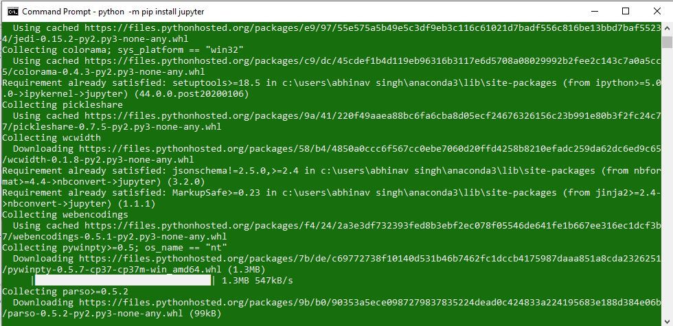
pip install notebookThis command tells PIP to install the ‘notebook’ package containing the classic Jupyter Notebook application.
- Verify the Installation: After the installation completes, you can verify it by running:
jupyter notebook --versionThis command would print the installed version of Jupyter Notebook if the installation were successful.
- Launch Jupyter Notebook: You can start the Jupyter Notebook interface in your browser by running:
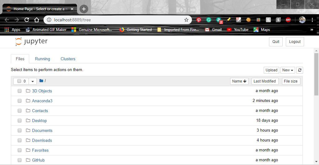
jupyter notebookThis command will print information about the notebook server in your terminal, including the web application URL (by default, http://localhost:8888).
Upon launching, your default browser should automatically open to this URL. You can manually open this URL in your browser if it doesn’t.
You might be interested in installing Jupyter Notebook in the Docker container. Check the How to build Anaconda Python Data Science Docker container for more information on this topic. Also, you might be interested in how to launch Nginx Jupyter Behind A Proxy Setup article, which covers Jupyter Hub installation.
You’ve now installed Jupyter Notebook! You’re ready to start creating and running your notebooks. In the next section, we’ll guide you on running your first Jupyter Notebook, where we’ll include some Python scripting examples.
Let’s continue our journey!
Running Your First Jupyter Notebook
Congratulations on successfully installing Jupyter Notebook! Now, let’s walk through creating and running your first notebook.
- Launch Jupyter Notebook: If you’ve closed it, relaunch Jupyter Notebook by running
jupyter notebookit in your terminal or command prompt. This command will open the Jupyter Notebook interface in your default web browser. - Create a new Notebook: In the Jupyter Notebook interface, navigate to the right-hand side of the screen and click on the ‘New’ button. Then, select ‘Python 3’ from the dropdown list. A new tab will open with your fresh notebook.
- Understanding the Interface: Each Jupyter Notebook is composed of cells. A cell is a multiline text input field, and its contents can be executed by using Shift-Enter, or by clicking either the “Play” button in the toolbar or Cell > Run in the menu bar. The cell’s type determines the execution behavior of a cell. There are three types of cells: code cells, markdown cells, and raw cells. In most cases, you’ll be working with code and markdown cells.
- Running Python Code: Click on the first cell and try typing some Python code, such as:
print("Hello, Jupyter!")Hit ‘Shift + Enter’ to run the cell. The output of the cell will appear below the code.
- Writing Markdown Text: You can use Markdown cells to explain your code and findings. Markdown is a lightweight markup language for creating formatted text. To create a Markdown cell, click on a cell, go to the ‘Cell’ menu, select ‘Cell Type’, and then ‘Markdown’. Now, you can write text in this cell. Try typing some text and then run the cell as you did before.
- Saving Your Notebook: To save your work, go to ‘File’ and then ‘Save and Checkpoint’, or just hit ‘Ctrl + S’.
You’ve created and run your first Jupyter Notebook. In the following sections, we’ll explore how to troubleshoot the Jupyter Notebook’s common installation issues effectively. Let’s proceed!
Troubleshooting Common Installation Issues
Like any software installation, you may encounter some challenges when installing Python or Jupyter Notebooks. Here are some common issues you might face and solutions to get you past them.
- Python not recognized as a command: If you see a ‘Python is not recognized as an internal or external command’ error after installing Python, this likely means that Python was not added to your system’s PATH. To fix this, you can manually add Python to your PATH variable. The method varies between operating systems and versions, so a quick internet search with your specific OS will provide the most accurate steps.
- PIP not working: If you’re having trouble using pip, it might be that pip isn’t installed, or it’s an issue with your PATH variable. Python 3 comes with pip preinstalled, so make sure you’re using Python 3. If you still have issues, try reinstalling Python and ensure the ‘pip’ box is checked during installation.
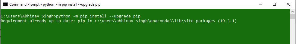
- Issues installing Jupyter Notebook: If you’re encountering errors while installing Jupyter Notebook, it might be due to an older version of PIP or Python. Make sure both are up-to-date. You can update pip by running
pip install --upgrade pipand update Python by downloading the latest version from the Python website. - Jupyter command not found: If you have installed Jupyter Notebook, but your system can’t seem to find it (i.e., you see a ‘jupyter: command not found’ error), this is likely because the location where pip installed Jupyter is not on your system’s PATH. As mentioned above, you can resolve this by adding the installation location to your PATH.
- Issues running Jupyter Notebook: If Jupyter Notebook doesn’t launch automatically, manually launch it by entering the URL in the terminal (usually http://localhost:8888) into your browser’s address bar. If the interface is still not showing up, ensure no firewall or security software is blocking Jupyter Notebook.
Remember, it’s okay to encounter problems during the installation process. It’s part of the learning experience. Don’t hesitate to search online for the errors you’re seeing – it’s likely that others have encountered the same issues and found solutions. Happy troubleshooting!
Best Practices for Using Jupyter Notebook with Python
Utilizing Jupyter Notebook effectively can make your Python programming more efficient and enjoyable. Here are some best practices to ensure you’re getting the most out of your Jupyter Notebook experience:
- Organize Your Code with Cells: Jupyter Notebook’s cell structure is its biggest strength. Make good use of it by organizing your code into logical sections. Each cell should accomplish a specific task or represent a specific step in your analysis or modeling process.
- Comment Your Code: Like any other programming environment, commenting on your Python code in Jupyter Notebooks is a good habit. Even though you can write rich text in markdown cells, inline comments in your code cells can provide context directly tied to the code.
# Calculate the sum of the list
sum_list = sum(my_list)- Use Markdown Cells for Documentation: Markdown cells are perfect for documenting your analysis process, explaining your reasoning, noting observations, and providing another context. This is what makes Jupyter Notebook great for data storytelling.
- Show Your Work: Jupyter Notebook allows you to display your Python data structures in a readable format. This feature shows intermediary steps in your data analysis or modeling process. This can be especially useful for debugging and explaining your process to others.
# Display the content of the list
print(my_list)- Keep Your Notebooks Reproducible: Try to keep your notebooks self-contained and reproducible. If someone else were to run your notebook, they should get the same results. This might involve setting seeds for random number generators, making sure any data files you use are accessible, and providing explicit instructions for any manual steps.
- Regularly Save Your Work: Jupyter automatically saves your notebook every few minutes, but you should also get into the habit of manually saving your work. You can do this by clicking ‘File’ > ‘Save and Checkpoint’, or by simply pressing ‘Ctrl + S’.
- Clear Your Output: When sharing your notebook, it can be helpful to clear your output data first. This makes the notebook smaller and encourages others to run the code themselves. You can clear output via ‘Cell’ > ‘All Output’ > ‘Clear’.
- Use Jupyter Extensions: Jupyter has many extensions that add useful functionality. These can be installed with pip and activated in Jupyter. For instance, the
nbextensions_configuratorextension provides a convenient way to configure and manage your Jupyter extensions.
Applying these best practices makes your Jupyter Notebook usage more efficient and productive. Happy coding!
FAQ
How do I install a Jupyter Notebook?
To install Jupyter Notebook, you must first install Python on your system. Python comes pre-installed on most UNIX-like systems, including Linux and MacOS. You can download Python from the official website if it’s not installed or using Windows. Once Python is installed, you can install Jupyter Notebook using Python’s package manager, pip. Open your system’s command prompt or terminal and type pip install notebook. Once the installation is complete, you can start Jupyter Notebook by typing jupyter notebook in the terminal. This command will launch the Jupyter Notebook interface in your default web browser, and you’re ready to create and share your interactive documents.
Do I need Python to install Jupyter Notebook?
Python is required to install Jupyter Notebook. Jupyter Notebook is written in Python, and its default kernel runs Python code. Therefore, you must install Python on your system before installing Jupyter Notebook. If Python is not installed, it can be downloaded from the official website. Once Python is installed, Jupyter Notebook can be easily installed using Python’s package manager, pip. It’s important to note that although Jupyter Notebook is Python-based, it can also run code from several other programming languages as long as the appropriate kernels are installed.
How to install Jupyter Notebook using Anaconda Mac?
Installing Jupyter Notebook on a Mac using Anaconda is a straightforward process. First, download the Anaconda installer for Mac from the official Anaconda website. Make sure to download the Python 3.x version. Once the installer is downloaded, open it and follow the on-screen instructions. Anaconda will install Python, Jupyter Notebook, and other useful data science packages. After the installation, you can launch Jupyter Notebook by opening the Anaconda Navigator application, which is installed as part of Anaconda, and then clicking on the Jupyter Notebook icon. Alternatively, you can open a terminal and type jupyter notebook to start Jupyter Notebook. This command will open a new tab in your default web browser with the Jupyter Notebook interface.
How to install Jupyter on Windows Terminal?
First, ensure Python is installed on your Windows system. If not, download it from the official Python website and include Python in the PATH during installation. Next, install Jupyter Notebook via Python’s package manager, pip. To do this, open Windows Terminal (accessed by typing ‘cmd’ in the search bar) and type pip install notebook. After the installation, launch Jupyter Notebook by entering jupyter notebook in the terminal. This command opens the Jupyter Notebook interface in your default web browser, ready for use.
how to install Jupyter Notebook in Windows 10?
To install Jupyter Notebook on Windows 10, you’ll first need to install Python, which can be downloaded from the official Python website. Ensure to check the box to add Python to your PATH during installation. After installing Python, open Command Prompt and type pip install notebook to install Jupyter Notebook using pip, Python’s package manager. After the installation, launch Jupyter Notebook by typing jupyter notebook into the Command Prompt. This command will open the Jupyter Notebook interface in your default web browser, ready for you to create and share interactive documents.
Conclusion
In this comprehensive guide, we’ve covered everything you need to know to install and get started with Jupyter Notebook. Beginning with the fundamentals of Jupyter Notebook, we delved into its prerequisites and guided you through the installation of Python and Jupyter Notebook. We also explored the creation of a Python virtual environment and guided you through running your first Jupyter Notebook.
Additionally, we touched on the collaboration and interactivity features of Jupyter Notebook, showcasing how they can enhance your programming and data analysis tasks. We provided solutions to common installation issues and shared best practices for using Jupyter Notebook with Python, aiming to optimize your Jupyter Notebook experience.
The world of programming is vast and continually evolving. As you advance your journey with Python and Jupyter Notebook, always remember to learn, explore, and experiment, but most importantly, have fun. Happy coding!
References and Additional Resources
To supplement your learning and explore more about Python, and Jupyter Notebook, refer to the following resources:
Python:
- Python Official Documentation
- Python for Beginners
- Learn Python – Full Course for Beginners by FreeCodeCamp
Jupyter Notebook:
- Jupyter Notebook Official Documentation
- Project Jupyter
- Jupyter Notebook Tutorial: Introduction, Setup, and Walkthrough by Corey Schafer
These resources should provide a good starting point for further exploration and mastery. Happy learning!
I’m a passionate Cloud Infrastructure Architect with more than 20 years of experience in IT. In addition to the tech, I’m covering Personal Finance topics at https://amaksimov.com.
Any of my posts represent my personal experience and opinion about the topic.