OSPF расшифровывается как Open Shortest Path First. Если переводить дословно, получится что-то вроде «открытый короткий путь первым». Под названием скрывается протокол внутренней маршрутизации, который передает информацию по лучшему пути. Но, несмотря на название, он не всегда короткий. Чтобы найти лучший путь, протокол отслеживает состояние каналов, а путь рассчитывается по алгоритму Дейкстры.
OSPF довольно просто настраивается по инструкциям, но вот объяснить порядок его работы довольно сложно. Попробуем это сделать.
Основы протокола OSPF
Чтобы объяснить работу OSPF-протокола, сначала вспомним, что такое статическая маршрутизация. Представим небольшую компанию с внутренней базой знаний, которая хранится на сервере в соседнем помещении. Когда сотрудник хочет открыть документ из базы, пакет с запросом передается на маршрутизатор. Последний обращается к таблице маршрутизации и понимает, в какую сеть отправить пакет.
Для этого администратор вручную прописывает все маршруты к сетям в таблице маршрутизации. Но когда в компании десяток департаментов и сотни маршрутизаторов, такой сценарий нереализуем (особенно при добавлении новых маршрутизаторов). Здесь на помощь приходит динамическая маршрутизация с помощью протокола OSPF.
Протокол OSPF заполняет таблицы маршрутизации автоматически, при этом маршрутизаторы постоянно обмениваются данными о состоянии сети и актуализируют таблицу. Администратору не нужно бегать и самостоятельно переписывать таблицы.
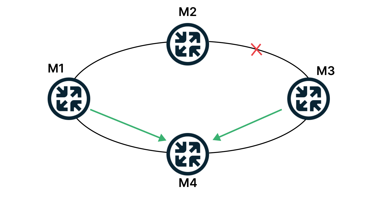
Аналогично в случае сбоев: со статической маршрутизацией тяжело отслеживать доступность сетей. Если канал между маршрутизаторами прерван, то пакеты, которые M2 получил от M1 (см. схему ниже), никуда не отправятся.
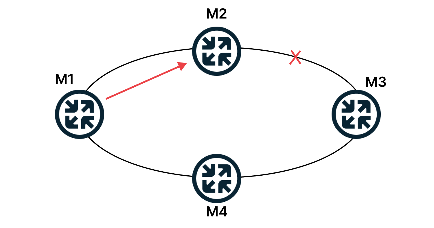
Если сети работают на протоколе OSPF, маршруты перестроятся автоматически.
OSPF — протокол внутренней маршрутизации. «Внутренней» означает, что маршрутизаторы связаны в замкнутой системе или в одном домене. Понимание принципов работы протокола и алгоритмов облегчат настройку OSPF, поэтому о них подробнее.
Терминология
- Автономная система — это сети под общим управлением, с едиными политиками маршрутизации для всех устройств.
- Интерфейс — соединение маршрутизатора и сети. В контексте OSPF термины «интерфейс» и «канал» (link) синонимичны.
- Area, или зона, — это условная «площадка» в виде комплекса маршрутизаторов, которые обмениваются LSA друг с другом. У маршрутизаторов в этой зоне единый идентификатор.
- LSA, или Link State Advertisement, — это сообщение (объявление, пакеты) о состоянии канала между маршрутизаторами. В нем содержатся данные о каналах маршрутизатора и их состоянии — например, прерывании, маршруте, интерфейсах.
- Состояние канала, или Link State, — состояние канала между двумя маршрутизаторами, которое обновляется посредством пакетов LSA.
- LSU, или Link State Update, — это пакет, в котором передается LSA (один или несколько).
- Link-State DataBase — это база сообщений LSA, в ней содержатся все записи о состоянии каналов. Встречается также термин «топологическая база данных» (topological database), это синоним.
- Router ID — индивидуальный и уникальный номер маршрутизатора для идентификации. Чаще всего это сетевой адрес интерфейса — 32-х битный номер.
- Маршрутизаторы, у которых интерфейс в одной зоне, называются соседями. Список всех соседей содержится в базе данных соседей.
- Для определения соседа маршрутизаторы обмениваются hello-сообщениями, или hello-пакетами. В hello-сообщениях содержатся LSA.
- Состояние смежности, или Adjacency, — взаимосвязь между определенными соседними маршрутизаторами для обмена информацией о маршрутах.
- Shortest Path First — алгоритм, который рассчитывает лучший маршрут между сетями.
- Стоимость — это условный показатель «цены» пересылки данных по каналу. В OSPF стоимость зависит от разных факторов — например, пропускной способности канала.
- Designated Router (DR) — выделенный маршрутизатор. Каждый маршрутизатор устанавливает с ним отношения, потому что DR управляет рассылкой LSA в сети и отправляет информацию остальным об изменениях в сети.
- Backup Designated Router (BDR) — резервный выделенный маршрутизатор. Маршрутизатор на случай выхода DR из строя. Каждый маршрутизатор в сети также устанавливает с ним отношения.
Алгоритм работы протокола OSPF
Примечание. Здесь мы изначально считаем, что на маршрутизаторе и интерфейсе установлен и включен OSPF.
Как работает динамическая маршрутизация OSPF? Краткое описание:
- Когда маршрутизатор включают, он выбирает Router ID, либо администратор устанавливает его значение вручную.
- Протокол ищет другие маршрутизаторы — подключенных соседей, отправляя им через определенные промежутки времени hello-пакеты с информацией о соседях и состоянии каналов.
- Если маршрутизатор получает в ответ пакет по интерфейсу, на которых активирован OSPF, то устанавливает с ним «соседские» отношения. Если не получает, маршрутизатор считает устройство «мертвым» — не отправляет ему трафик и перестраивает маршруты.
- После того как маршрутизаторы подружились, они обмениваются LSA-сообщениями о подключенных и доступных сетях, о соседском роутере и стоимости. Эти данные нужны, чтобы построить карту сети (топологию) — она пригодится для расчетов кратчайшего пути трафика. Карта одинакова на всех маршрутизаторах.
- Маршрутизаторы синхронизируют общую базу LSDB, где хранят LSA.
- В сети могут быть сотни или тысячи маршрутизаторов. Отправка сообщений LSA от каждого устройства к каждому обязательно забьет каналы. Чтобы этого не произошло, отправкой сообщений заведует DR: через него отправляется информация об изменениях в сети ко всем маршрутизаторам — например, когда какой-то маршрутизатор упал. Если DR не прописан изначально, то им становится маршрутизатор с самым большим IP-адресом.
- Дальше запускается алгоритм SPF, который рассчитывает оптимальный маршрут к каждой сети. Процесс похож на построение дерева, где корень — маршрутизатор, а ветви — пути к доступным сетям. В общей таблице маршрутизации будут храниться лучшие пути к каждой сети.
Теперь подробнее о каждом этапе.
Запуск протокола
Для запуска OSPF-протокола нам нужно запустить процесс OSPF на маршрутизаторе подобной командой:
selectel-gw1(config)# router OSPF 1Мы сообщаем, что запускаем протокол, указываем, какой именно, уточняем номер процесса (в конце).
Автоматически назначается Router ID. По умолчанию это наибольший IP-адрес устройства. Но можно настроить идентификатор вручную:
selectel-gw1(config-router)#router-id 172.16.255.1Следующим шагом объявляем, какие сети будем передавать соседям OSPF. С помощью этой команды сообщаем, с каких интерфейсов будут отправляться hello-пакеты и какие сети хотим анонсировать другим маршрутизаторам:
selectel-gw1(config-router)#network 172.16.0.0 0.0.255.255 area 0Первый параметр — номер сети, второй — wildcard-маска, последний — номер зоны.
Готово! Если другие роутеры в сети настроены, то они установят соседские отношения.
Примечания. На соседских маршрутизаторах должны совпадать интервалы hello-пакетов, Dead Interval, интерфейсы и номера зон.
Установка отношений соседства
Если есть Router ID, совпадают интерфейсы, запущен OSPF-протокол и указаны сети, которые необходимо анонсировать по OSPF, то маршрутизаторы установят отношения соседства и произойдет обмен маршрутов.
Установка отношений происходит в несколько этапов. Рассмотрим на примере, когда у нас есть четыре маршрутизатора M1, M2, M3 и M4, который считаем новым. При этом M2 выбран как DR, а M3 как BDR.
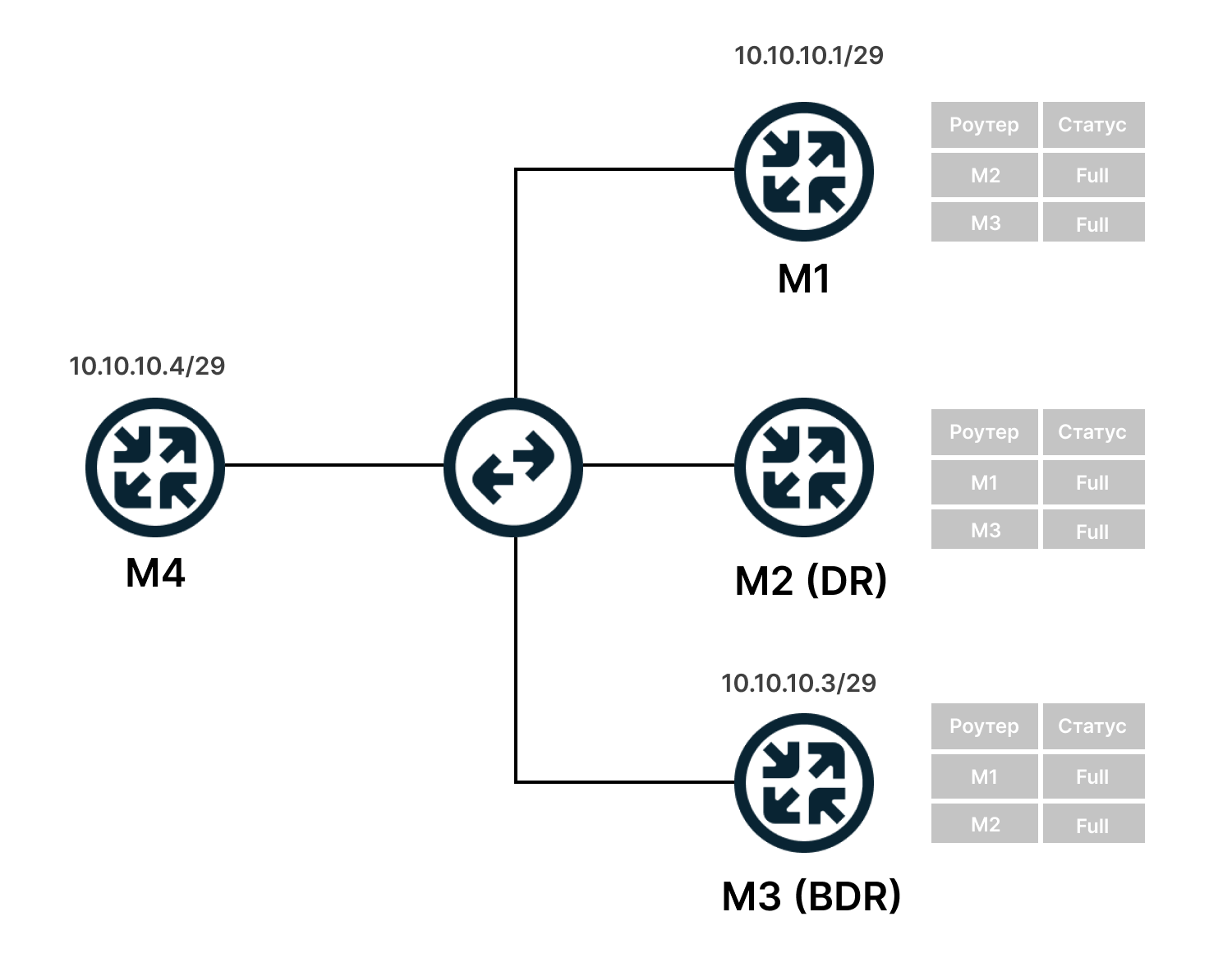
- Маршрутизатор M4 рассылает hello-сообщения на групповой адрес 224.0.0.5.
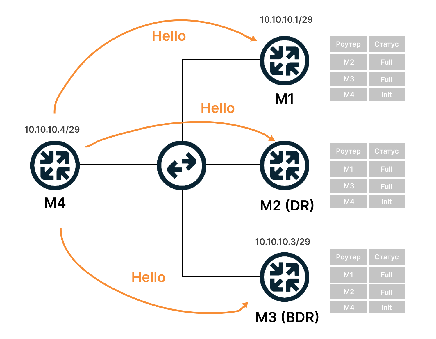
- Маршрутизаторы M1, M2 и M3 получили сообщения и добавили M4 в список соседей. Его статус они определяют как Init (состояние попытки поиска).
- Маршрутизаторы M1, M2, M3 отправляют сообщения маршрутизатору M4 с его Router ID и списком соседей. M4 добавляет их в список соседей.
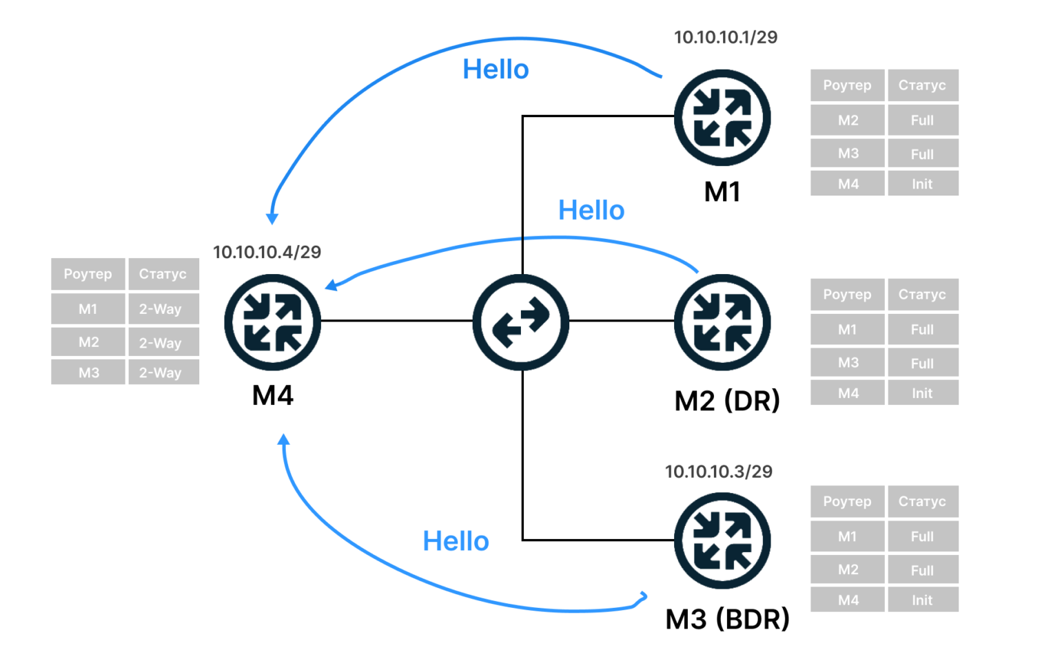
- Устанавливаются симметричные соседские отношения 2-Way (состояние, когда есть обмен сообщениями, но без передачи маршрутов).
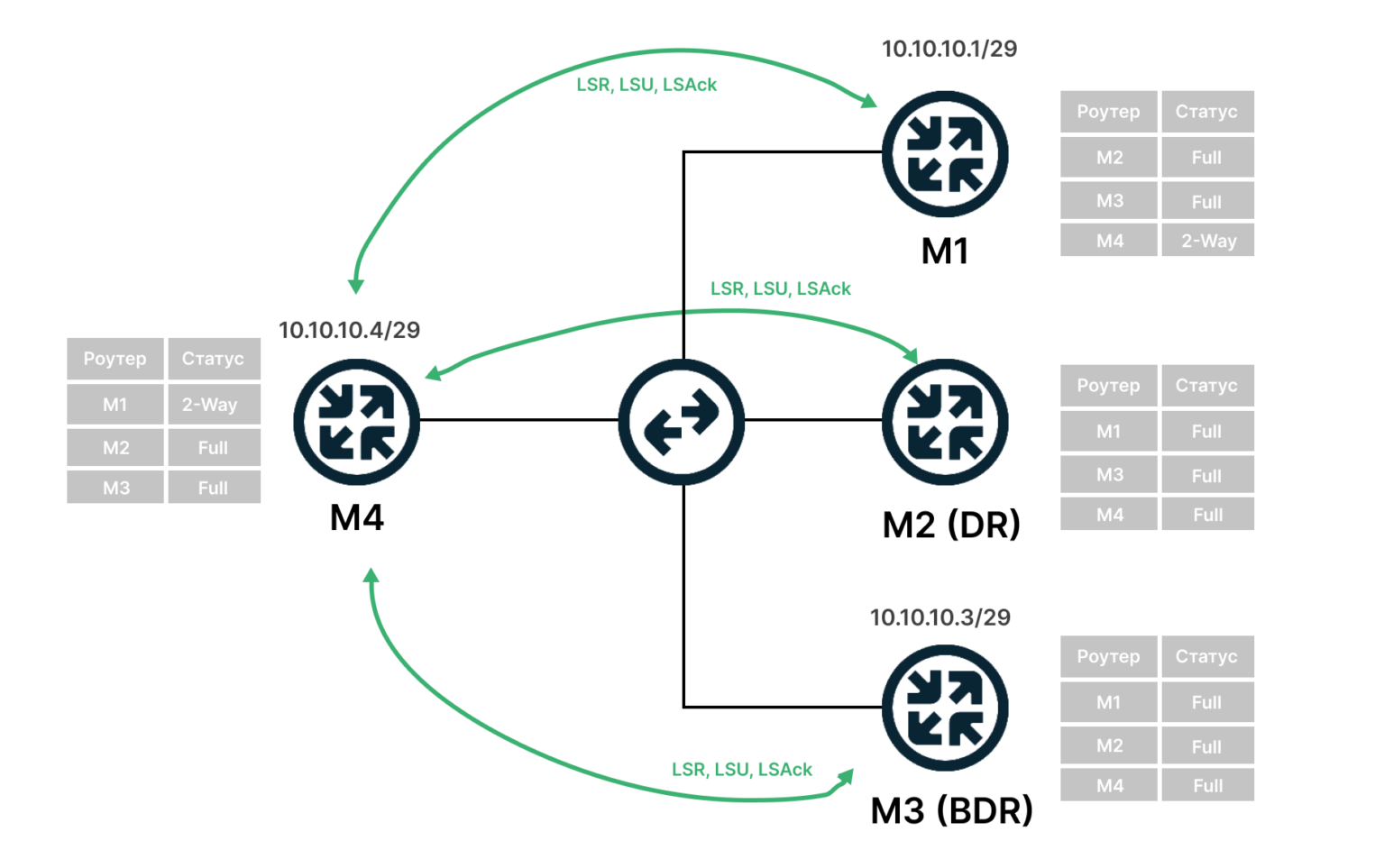
- Устройства обмениваются служебными сообщениями с кратким описанием базы данных маршрутов и LSR-сообщениями (Link State Request), запросами о неизвестных сетях.
- Устройства обмениваются сообщениями с более подробным описанием маршрутов и синхронизируют LSDB. Статус отношений устанавливается в Full, передаются маршруты.
Отношения соседства устанавливаются со всеми маршрутизаторами, включая DR и BDR.
Распределение ролей
Выше мы писали, что в сети назначаются две важные роли:
- Designated Router (DR) — выделенный маршрутизатор,
- Backup Designated Router (BDR) — резервный выделенный маршрутизатор.
DB и BDR назначаются администратором вручную или автоматически во время установления отношений соседства. Вручную обычно DR/BDR ставят корневые, а автоматически выбирается маршрутизатор с самым высоким приоритетом интерфейса OSPF или с наибольшим Router ID. BDR выбирается второй маршрутизатор по приоритету. Когда DR выходит из строя, то его заменяет BDR. Далее проводится выбор нового BDR.
Обе роли нужны, чтобы уменьшить количество LSA-сообщений. Работает это так.
Маршрутизаторы обмениваются маршрутной информацией и отправляют сообщения об изменениях в сети в DR. Он, в свою очередь, отправляет информацию остальным. Каждый маршрутизатор в сети также устанавливает с ним отношения, потому что фактически все маршрутизаторы устанавливают отношения друг с другом через DR.
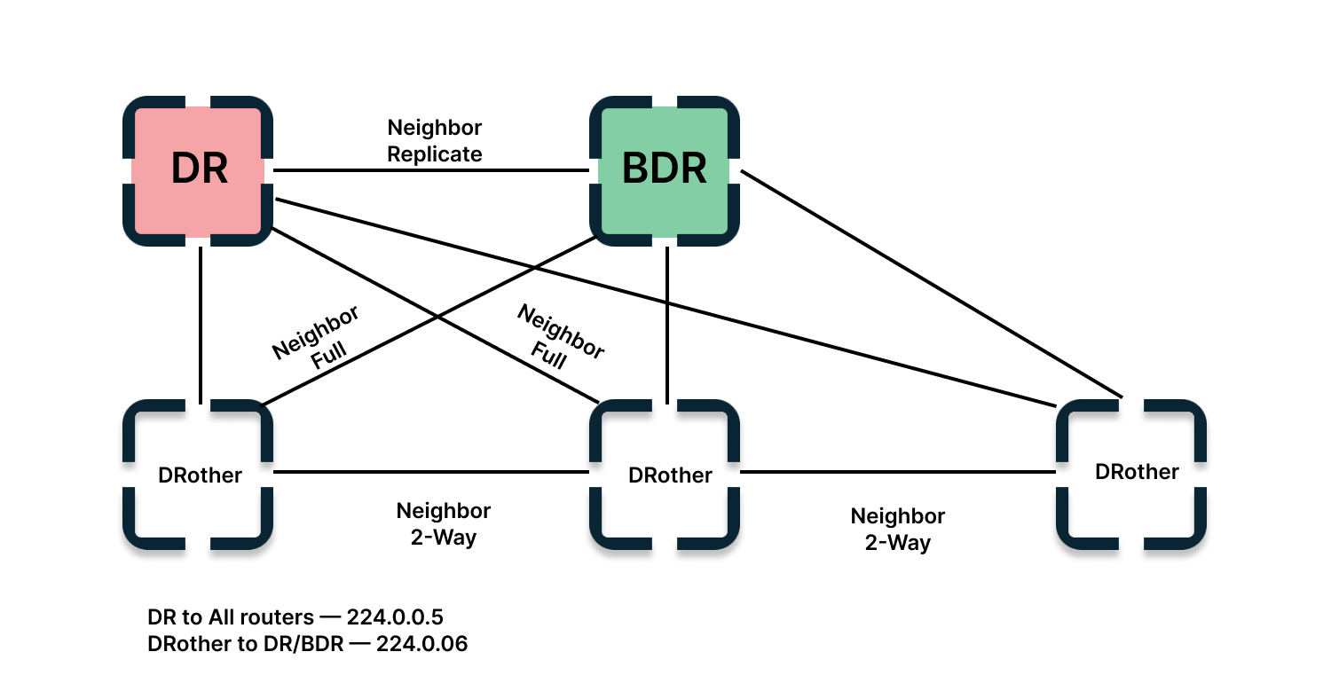
После выбора DR соседи обмениваются DBD-сообщениями — они содержат описание LSDB (Link-State DataBase), чтобы синхронизироваться. Для этого за устройствами DR и BDR закрепляется групповой адрес — например, 224.0.0.5, как на схеме выше.
Зоны OSPF: магистральная, стандартная, NSSA, stub area
OSPF позволяет делить сеть на зоны — логические объединения узлов и сетей. Зона — это набор маршрутизаторов со своей базой, LSA, топологией. Маршрутизаторы другой зоны не знают о топологии других зон. У каждой зоны есть свой идентификатор — area ID. Идентификатор может быть указан в формате IP-адреса, но это не IP-адреса. Идентификация маршрутизаторов зоны проходит с помощью Router ID.
В OSPF есть несколько зон.
Магистральная (Area 0, Backbone-area, зона 0.0.0.0). Она особенная — формирует ядро сети OSPF. Все остальные зоны подключаются к ней. Все пакеты от любой ненулевой зоны в другую ненулевую проходят через магистральную. Магистральный маршрутизатор — Backbone Router, у которого хотя бы один интерфейс принадлежит магистральной зоне.
Стандартная (обычная, Normal). Это область без определенной цели: создается по умолчанию, принимает обновления каналов, суммарные и внешние маршруты.
Транзитная. Зона, которая используется для передачи сетевого трафика из одной смежной области в другую. Магистральная зона, например, тоже транзитная, но особого типа.
NSSA (Not-so-stubby area). Это специфичная область, которая может инжектировать внешние маршруты сообщений в систему с помощью специального типа LSA и отправлять их в другие области. Но зона не может получать внешние маршруты из других областей.
Для передачи данных в этой зоне используется маршрутизатор ASBR, Autonomous System Boundary Router. Он применяется не только здесь, а, в целом, для получения маршрутов из внешних систем. Для передачи данных на границах зон используются пограничные маршрутизаторы ABR, или Area Border Router.
Тупикова зона (stub area). Эта зоне не принимает информацию о внешних маршрутах для автономной системы, но принимает маршруты из других зон. В тупиковой зоне не может находиться ASBR. Для передачи сообщений за границу системы из тупиковой зоны маршрутизаторы используют маршрут по умолчанию.
Также есть totally stub area — это «усиление» тупиковой зоны (термин внедрен компанией Cisco). В отличие от stub area в ней заменены на маршрут по умолчанию и внешние, и межзональные маршруты.
Все маршрутизаторы, которые находятся внутри зон (магистральной тоже), называются Internal Router — внутренними. Их интерфейсы принадлежат одной зоне. У таких маршрутизаторов только одна база данных состояния каналов.
Примечание. Маршрутизаторы могут выполнять несколько функций/ролей одновременно.
Зона не обязательно должны быть физической — соединение может быть установлено и с помощью виртуальных каналов.
Мультизона и ее преимущества
Мультизона, или мультизональность, удобна при большом количестве маршрутизаторов. Разделение позволяет:
- Сегментировать сеть, например, по отделам или департаментам.
- Снизить нагрузку на ЦПУ маршрутизаторов, потому что уменьшается количества перерасчетов по алгоритму SPF. Например, делим 100 роутеров на три зоны. При падении одного из них маршрут перестраивается не для всех, а лишь для трети роутеров.
- Снизить размер таблиц маршрутизации, потому что маршруты на границах зон суммируются.
- Снизить число пакетов LSA.
Объявления о состоянии канала — LSA
LSA, или Link State Advertisement, — это сообщение с описанием локального состояния маршрутизатора или сети. Вместе они создают базу данных состояния каналов LSDB. Есть 11 типов LSA сообщений (пакетов), у каждого своя функция.
Рассмотрим каждый LSA type.
LSA 1 (Router LSA). Каждый маршрутизатор создает этот тип. Он отправляется между маршрутизаторами одной зоны и дальше не идет. Содержит описание интерфейсов, как соединены маршрутизаторы и сети внутри зоны.

LSA 2 (Network). Этот тип рассылается между соседями в одной зоне, а создает его DR для описания маршрутизаторов, которые подключены к нему.

LSA 3 (Summary, Network Summary). Эти сообщения (пакеты) создает ABR, чтобы передать информацию о маршрутах соседей (из первого и второго типов) в другую область, в сокращенном виде. В сообщениях описываются подсети, стоимость маршрута, но не топология зоны.

LSA 4 (ASBR Summary). Как третий тип, но передает маршрут до локального ASBR соседям из других зон.

LSA 5 (External) содержат информацию из внешних систем — например, из другого протокола. Сообщения создает ASBR.
LSA 6 (Group Membership LSA) разработаны для протокола Multicast OSPF (MOSPF) , который поддерживает многоадресную маршрутизацию через OSPF. Не поддерживается Cisco.
LSA 7 (NSSA External) как пятый тип, но создает ASBR, если он находится в зоне NSSA.
Тип LSA 8 используется для передачи атрибутов BGP через сеть OSPF, а специальные типы LSA с 9 до 11 — специальные, используются для расширения возможностей, например, потоковой передачи данных.
Типы пакетов OSPF
LSA сами по себе не передаются. Маршрутизаторы передают LSA внутри других пакетов. Например, LSU или DD (Database Description), где передается описание всех LSA, которые хранятся в LSDB маршрутизатора. Кроме них, в OSPF используется еще три типа пакетов: Hello, Link-State Request (LSR) и Link-State Acknowledgment (LSAck).
В заголовке любого OSPF-пакета передается такая информация:
- Version — номер версии протокола OSPF.
- Type — тип OSPF-пакета, например, Hello.
- Packet length — длина пакета с заголовком в байтах.
- Router ID — идентификатор маршрутизатора.
- Area ID — 32-битный идентификатор зоны, определяет, в какой зоне создан пакет.
- Checksum — контрольная сумма, для проверки целостности пакета.
- Authentication type — тип используемой схемы аутентификации. Есть три типа: 0 (нет), 1 (есть аутентификация), 2 (MD5-аутентификация).
- Authentication — поле данных аутентификации.
Каждый тип пакета передает еще дополнительную информацию, кроме общей.
Hello. Пакеты передаются маршрутизаторами для обнаружения соседей, подтверждения их работы и построения отношения.
Пакет выглядит примерно так.
В сообщении передаются параметры, о которых маршрутизаторы должны договориться перед тем, как станут соседями.
- Network mask — сетевая маска интерфейса.
- HelloInterval — информация о частоте отправки.
- Options — дополнительные опции, которые поддерживает маршрутизатор, например, MC-bit.
- Router Priority — приоритет маршрутизатора. Эта информация используется при выборе DR и BDR.
- RouterDeadInterval — интервал времени, после которого сосед считается «мертвым».
- Designated Router — IP-адрес DR для сети, в которую отправлен hello-пакет.
- Backup Designated Router — IP-адрес BDR.
- Neighbor — идентификаторы соседей-маршрутизаторов.
Database Description (DBD). Проверяет синхронизацию базы данных между маршрутизаторами. В пакете содержатся данные:
- Interface MTU — максимальный размер в байтах IP-дейтаграммы, которая может быть отправлена через интерфейс без фрагментации.
- I-бит — устанавливается для первого пакета в последовательности.
- M-бит — указывает наличие последующих дополнительных пакетов.
- MS-бит — устанавливается для ведущего.
- DD sequence number — уникальное значение, устанавливается в начальном пакете; в каждом следующем увеличивается на единицу, пока не будет передана вся база данных.
- LSA headers — массив заголовков базы данных состояния каналов.
Link-State Request (LSR). Предназначен для запроса части базы данных соседнего маршрутизатора. В пакете содержатся.
- LS Type — тип сообщения.
- Link State ID — идентификатор домена маршрутизации.
- Advertising Router — идентификатор маршрутизатора, который создал объявление о состоянии канала.
Link-State Update (LSU). Предназначен для рассылки записей о состоянии каналов. В нем содержится Number of LSA — количество объявлений в пакете.
Link-State Acknowledgment (LSAck). Сообщение, которое подтверждает получение других типов пакетов.
Синхронизация LSDB
Все LSA всех типов образуют LSDB. У каждого маршрутизатора есть своя копия LSDB и они синхронизируют свою LSDB с DR.
- Каждый маршрутизатор отвечает за записи в LSDB о связях, которые исходят от него.
- Когда появляется новая связь или происходит обрыв, маршрутизатор меняет свою копию базы и извещает DR.
- Остальные будут забирать данную информацию с DR.
За извещение отвечает Flooding protocol — все маршрутизаторы пересылают сообщения об обновлении состояния связей (LSA). Получение подтверждается сообщениями LSA с типом OSPF, о котором говорили выше. У каждой записи в LSDB есть номер версии. У следующей записи номер больше, чем у предыдущей, чтобы в базу не попадали устаревшие версии.
Выбор лучшего маршрута
За выбор лучшего маршрута отвечает алгоритм SPF. Например, у нас есть сеть в виде графа, в узлах которой маршрутизаторы, а за ними сети. Как выбрать маршрут передачи данных?
У каждого ребра — пути между соседними маршрутизаторами — есть стоимость. Чтобы рассчитать маршрут, нужно знать всю топологию сети: каждый маршрутизатор передает друг другу знания о соседях, соединении и его стоимости.
Когда топология известна, проводится расчет по алгоритму Дейкстры (SPF) — нидерландского ученого, который разработал его еще в 1959 году. Маршрутизатор выбирает маршрут на основании наименьшего значения стоимости пути.
Стоимость рассчитывается по нескольким метрикам. Метрикой может быть загрузка канала, задержка, надежность связи или полоса пропускания канала. Например, последнюю метрику производители устройств считают каждый по своему: для маршрутизаторов Cisco это время передачи 100 Мбит данных по каналу в секундах.
Также у маршрута есть приоритет (в порядке убывания):
- Внутренние маршруты зоны.
- Маршруты между зонами.
- Внешние маршруты.
Выбирая путь, маршрутизатор будет выбирать сначала приоритетные маршруты. В первую очередь учитываются связи между маршрутизаторами и транзитными сетями, потом включаются тупиковые ветви, дальше — межзональные маршруты и маршруты к внешним сетям.
После расчета маршрутов создается дерево SPF.
Маршруты добавляются в таблицу маршрутизации.
Для получения маршрута маршрутизатор обращается к таблице LSDB. При этом таблица постоянно обновляется. Но обновление означает обнуление — маршруты строятся снова, с нуля, даже если изменились параметры всего одного маршрутизатора. Этот процесс сильно нагружает CPU.
От серверов до сетевых услуг и оборудования.
Реализации OSPF в Cisco и Juniper
Запуск и настройка OSPF протокола на оборудовании Cisco практически ничем не отличается от стандартного, описанного выше. Мы также включаем протокол на маршрутизаторах:
ter ospf 1Задаем Router ID, сеть и зоны:
router ospf 1
 router-id 1.1.1.1
 log-adjacency-changes
 redistribute static
 network 1.1.1.1 0.0.0.0 area 0
 network 172.16.1.0 0.0.0.255 area 0
!
Проверяем, заработала ли маршрутизация:
show ip ospf neighborsПроверяем таблицу маршрутизации:
show ip routeРеализация OSPF-протокола на устройствах Juniper аналогична, но команды другие. Включаем OSPF, определяем интерфейсы и зоны:
set protocols ospf area 0.0.0.0 interface ge-0/0/0.0
set protocols ospf area 0.0.0.0 interface ge-0/0/1.0
Здесь мы настроили область OSPF 0 (0.0.0.0) на интерфейсах ge-0/0/0.0 и ge-0/0/1.0 для маршрутизатора.
Для примера возьмем второй роутер:
set protocols ospf area 0.0.0.0 interface ge-0/0/0.0
set protocols ospf area 0.0.0.0 interface ge-0/0/2.0
Проверяем соседа:
root@R1> show ospf neighborУвидим подобный ответ — значит, сосед активен:
| Address | Interface | State | ID | Pri | Dead |
| 1.1.1.2 | ge-0/0/0.0 | Full | 1.1.1.2 | 128 | 39 |
Проверяем интерфейсы:
root@R1> show ospf interfaceПроверим маршруты, таблицу:
root@R1> show routeГотово.
OSPF для IPv6
IPv6 поддерживается протоколом OSPF, но только третьей версии. Версия OSPFv2 поддерживает только IPv4. При переходе на протокол OSPFv3 почти ничего не меняется — вся теория работает и на этой версии.
В целом, настройка выглядит примерно так же:
- Включаем OSPF.
- Задаем идентификатор маршрутизатора. В OSPFv3 Router ID. Для IPv6 он настраивается только вручную, если не настроен адрес IPv4.
Как это выглядит в виде команд:
ipv6 router ospf 1
 router-id 1.0.0.0
 exit

interface Serial0/0/0
 ipv6 ospf 1 area 0
 exit

interface Serial0/0/1
 ipv6 ospf 1 area 0
 exit
Команда для проверки базы LSDB:
show ipv6 ospf database
Команда проверки соседей:
show ipv6 ospf neighbor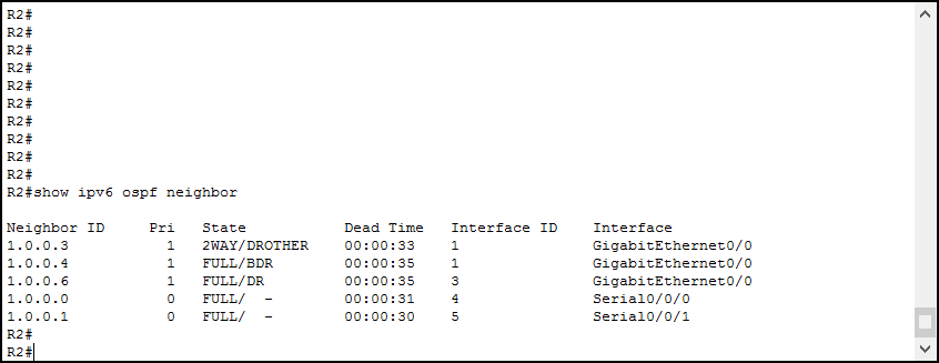
В контексте настроек OSPF для IPv6 остаются те же идентификаторы, те же области и зоны, так же настраиваются IP-адреса. При этом все маршрутизаторы Cisco поставляются с предварительно настроенными адресами IPv6.
Итог
OSPF — это открытый протокол для динамической маршрутизации внутренних сетей.
- Основа OSPF — протокол SPF, вычисляющий лучший (не кратчайший) маршрут.
- Для вычислений в протоколе реализована общая база маршрутов LSDB.
- База синхронизируется благодаря постоянным LSA сообщениям о состоянии каналов от маршрутизаторов.
- OSPF инкапсулируется в IP, без TCP/UDP, их замена — hello-сообщения.
- Hello-сообщения помогают реализовать отношения соседства и смежности с другими маршрутизаторами. Это позволяет протоколу проверять состояния канала и автоматически перестраивать маршруты, используя SPF-алгоритм.
- Перестройка маршрутов происходит локально, поэтому быстро, но затратно для процессора и оперативной памяти.
- Протокол поддерживает иерархические структуры зон, а значит — масштабирование.
- Есть несколько версий протокола, чаще используется вторая, а третья поддерживает IPv6.
Introduction
This document describes how OSPF works and how it can be used to design and build large and complicated networks.
Background Information
The Open Shortest Path First (OSPF) protocol, defined in RFC 2328, is an Interior Gateway Protocol used to distribute routing information within a single Autonomous System.
OSPF protocol was developed due to a need in the internet community to introduce a high functionality non-proprietary Internal Gateway Protocol (IGP) for the TCP/IP protocol family.
The discussion of the creation of a common interoperable IGP for the Internet started in 1988 and did not get formalized until 1991.
At that time, the OSPF Working Group requested that OSPF be considered for advancement to Draft Internet Standard.
The OSPF protocol is based on link-state technology, which is a departure from the Bellman-Ford vector based algorithms used in traditional Internet routing protocols such as RIP.
OSPF has introduced new concepts such as authentication of routing updates, Variable Length Subnet Masks (VLSM), route summarization, and so forth.
These chapters discuss the OSPF terminology, algorithm and the benefits and nuances of the protocol in the design of the large, complicated networks of today.
OSPF versus RIP
The rapid growth and expansion of modern networks has pushed Routing Information Protocol (RIP) to its limits. RIP has certain limitations that can cause problems in large networks:
- RIP has a limit of 15 hops. A network that spans more than 15 hops (15 routers) is considered unreachable.
- RIP cannot handle Variable Length Subnet Masks (VLSM). Given the shortage of IP addresses and the flexibility VLSM gives in the efficient assignment of IP addresses, this is considered a major flaw.
Periodic broadcasts of the full routing table consume a large amount of bandwidth. This is a major problem with large networks especially on slow links and WAN clouds.
- RIP converge is slower than OSPF. In large networks convergence gets to be in the order of minutes.
- RIP routers go through a period of a hold-down and garbage collection and slowly time-out information that has not been received recently. This is inappropriate in large environments and could cause routing inconsistencies.
- RIP has no concept of network delays and link costs. Routing decisions are based on hop counts. The path with the lowest hop count to the destination is always preferred even if the longer path has a better aggregate link bandwidth and less delays.
- RIP networks are flat networks. There is no concept of areas or boundaries. With the introduction of classless routing and the intelligent use of aggregation and summarization, RIP networks have fallen behind.
Enhancements were introduced in a new version of RIP called RIP2. RIP2 addresses the issues of VLSM, authentication, and multicast routing updates.
RIP2 is not a big improvement over RIP (now called RIP1) because it still has the limitations of hop counts and slow convergence which are essential in large networks.
OSPF, on the other hand, addresses most of the issues previously presented:
- With OSPF, there is no limitation on the hop count.
- The intelligent use of VLSM is very useful in IP address allocation.
- OSPF uses IP multicast to send link-state updates. This ensures less process resource consumption on routers that do not listen to OSPF packets. Updates are only sent in case routing changes occur instead of periodically. This ensures efficient bandwidth.
- OSPF has better convergence than RIP. This is because routing changes are propagated instantaneously and not periodically.
- OSPF allows for better load balancing.
- OSPF allows for a logical definition of networks where routers can be divided into areas. This limits the explosion of link state updates over the whole network. This also provides a mechanism to aggregate routes and decrease the unnecessary propagation of subnet information.
- OSPF allows for routing authentication through different methods of password authentication.
- OSPF allows for the transfer and tagging of external routes injected into an Autonomous System. This keeps track of external routes injected by exterior protocols such as BGP.
This leads to more complexity in the configuration and troubleshooting of OSPF networks.
Administrators that are used to the simplicity of RIP are challenged with the amount of new information they have to learn in order to keep up with OSPF networks.
This introduces more overhead in memory allocation and CPU utilization. Some of the routers which run RIP have to be upgraded in order to handle the overhead caused by OSPF.
What Do We Mean by Link-States?
OSPF is a link-state protocol. Think of a link as an interface on the router. The state of the link is a description of that interface and of its relationship to its neighbor routers.
A description of the interface would include, for example, the IP address of the interface, the mask, the type of network it is connected to, the routers connected to that network and so on.
The collection of all these link-states would form a link-state database.
Shortest Path First Algorithm
OSPF uses a shortest path first algorithm to build and calculate the shortest path to all destinations. The shortest path is calculated with the Dijkstra algorithm.
The algorithm by itself is complicated. This is a high level look at the various steps of the algorithm:
- Upon initialization or due to any change in routing information, a router generates a link-state advertisement. This advertisement represents the collection of all link-states on that router.
- All routers exchange link-states through floods. Each router that receives a link-state update must store a copy in its link-state database and then propagate the update to other routers.
- After the database of each router is completed, the router calculates a Shortest Path Tree to all destinations. The router uses the Dijkstra algorithm in order to calculate the shortest path tree, destinations, associated cost, and next hop to reach those destinations form the IP routing table.
- In case changes in the OSPF network do not occur, such as cost of a link or a network which is added or deleted, OSPF remains very quiet. Changes are communicated through link-state packets, and the Dijkstra algorithm is recalculated to find the shortest path.
The algorithm places each router at the root of a tree and calculates the shortest path to each destination based on the cumulative cost required to reach that destination.
Each router has its own view of the topology even though all the routers build a shortest path tree which uses the same link-state database. These sections indicate what is involved in the creation of a shortest path tree.
OSPF Cost
The cost (also called metric) of an interface in OSPF is an indication of the overhead required to send packets across a certain interface.
The cost of an interface is inversely proportional to the bandwidth of that interface. A higher bandwidth indicates a lower cost
There is more overhead (higher cost) and time delays involved through a 56k serial line than through a 10M ethernet line.
The formula used to calculate the cost is:
- cost= 10000 0000/bandwidth in bps
For example, it costs 10 EXP8/10 EXP7 = 10 to cross a 10M Ethernet line and 10 EXP8/1544000 = 64 to cross a T1 line.
By default, the cost of an interface is calculated based on the bandwidth; you can force the cost of an interface with the ip ospf cost <value> interface subconfiguration mode command.
Shortest Path Tree
Refer to this network diagram with the indicated interface costs. In order to build the shortest path tree for RTA, we would have to make RTA the root of the tree and calculate the smallest cost for each destination.
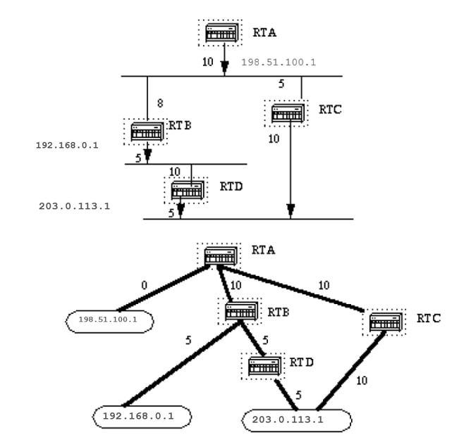
This is the view of the network as seen from RTA. Note the direction of the arrows in the cost calculation.
The cost of RTB interface to network 198.51.100.1 is not relevant when the cost is calculated to 192.168.0.1.
RTA can reach 192.168.0.1 via RTB with a cost of 15 (10+5).
RTA can also reach 203.0.113.1 via RTC with a cost of 20 (10+10) or via RTB with a cost of 20 (10+5+5).
In case equal cost paths exist to the same destination, the implementation of OSPF keeps track of up to six (6) next hops to the same destination.
After the router builds the shortest path tree, it builds the routing table. Directly connected networks are reached via a metric (cost) of 0 and other networks are reached in accord with the cost calculated in the tree.
Areas and Border Routers
As previously mentioned, OSPF uses floods to exchange link-state updates between routers. Any change in routing information is flooded to all routers in the network.
Areas are introduced to put a boundary on the explosion of link-state updates. Floods and calculation of the Dijkstra algorithm on a router is limited to changes within an area.
All routers within an area have the exact link-state database. Routers that belong to multiple areas, and connect these areas to the backbone area are called area border routers (ABR).
ABRs must therefore maintain information that describes the backbone areas and other attached areas.
An area is interface specific. A router that has all of its interfaces within the same area is called an internal router (IR).
A router that has interfaces in multiple areas is called an area border router (ABR).
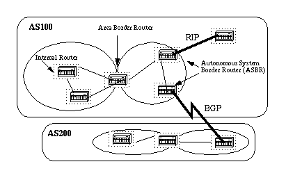
Routers that act as gateways (redistribution) between OSPF and other routing protocols (IGRP, EIGRP, IS-IS, RIP, BGP, Static) or other instances of the OSPF routing process are called autonomous system boundary router (ASBR). Any router can be an ABR or an ASBR.
Link-State Packets
There are different types of Link State Packets, those are what you normally see in an OSPF database (Appendix A and illustrated here).
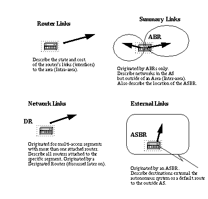
The router links are an indication of the state of the interfaces on a router in a certain designated area. Each router generates a router link for all of its interfaces.
Summary links are generated by ABRs; this is how network reachability information is disseminated between areas.
Normally, all information is injected into the backbone (area 0) and in turn the backbone passes it on to other areas.
ABRs also propagate the reachability of the ASBR. This is how routers know how to get to external routes in other ASs.
Network Links are generated by a Designated Router (DR) on a segment (DRs are discussed later).
This information is an indication of all routers connected to a particular multi-access segment such as Ethernet, Token Ring and FDDI (NBMA also).
External Links are an indication of networks outside of the AS. These networks are injected into OSPF via redistribution. The ASBR injects these routes into an autonomous system.
Enable OSPF on the Router
OSPF enable on the router involves two steps in config mode:
- Enable an OSPF process with the
router ospf <process-id>command. - Area assignment to the interfaces with the
network <network or IP address> <mask> <area-id>command.
The OSPF process-id is a numeric value local to the router. It does not have to match process-ids on other routers.
It is possible to run multiple OSPF processes on the same router, but is not recommended as it creates multiple database instances that add extra overhead to the router.
The network command is an assignment method of an interface to a certain area. The mask is used as a shortcut and it puts a list of interfaces in the same area with one line configuration line.
The mask contains wild card bits where 0 is a match and 1 is a «do not care» bit, for example, 0.0.255.255 indicates a match in the first two bytes of the network number.
The area-id is the area number we want the interface to be in. The area-id can be an integer between 0 and 4294967295 or can take a form similar to an IP address A.B.C.D.
Here is an example:
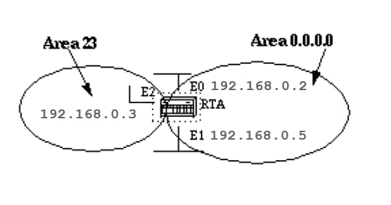
RTA#
interface Ethernet0
ip address 192.168.0.2 255.255.255.0

interface Ethernet1
ip address 192.168.0.5 255.255.255.0

interface Ethernet2
ip address 192.168.0.3 255.255.255.0

router ospf 100
network 192.168.0.4  0.0.255.255 area 0.0.0.0
network 192.168.0.3 0.0.0.0 area 23
The first network statement puts both E0 and E1 in the same area 0.0.0.0, and the second network statement puts E2 in area 23. Note the mask of 0.0.0.0, which indicates a full match on the IP address.
This is an easy way to put an interface in a certain area if you are are unable to resolve a mask.
OSPF Authentication
It is possible to authenticate the OSPF packets such that routers can participate in routing domains based on predefined passwords.
By default, a router uses a Null authentication which means that routing exchanges over a network are not authenticated. Two other authentication methods exist: Simple password authentication and Message Digest authentication (MD-5).
Simple Password Authentication
Simple password authentication allows a password (key) to be configured per area. Routers in the same area that want to participate in the routing domain has to be configured with the same key.
The drawback of this method is that it is vulnerable to passive attacks. Anybody with a link analyzer could easily get the password off the wire.
To enable password authentication, use these commands:
ip ospf authentication-key key(this goes under the specific interface)area area-id authentication(this goes underrouter ospf <process-id>)
Here is an example:
interface Ethernet0
ip address 10.0.0.1 255.255.255.0
ip ospf authentication-key mypassword

router ospf 10
network 10.0.0.0 0.0.255.255 area 0
area 0 authentication
Message Digest Authentication
Message Digest authentication is a cryptographic authentication. A key (password) and key-id are configured on each router.
The router uses an algorithm based on the OSPF packet, the key, and the key-id to generate a «message digest» that gets appended to the packet.
Unlike the simple authentication, the key is not exchanged over the wire. A non-decreasing sequence number is also included in each OSPF packet to protect against replay attacks.
This method also allows for uninterrupted transitions between keys. This is helpful for administrators who wish to change the OSPF password without communication disruption.
If an interface is configured with a new key, the router sends multiple copies of the same packet, each authenticated by different keys.
The router does not send duplicate packets when it detects that all of its neighbors have adopted the new key.
These are the commands used for message digest authentication:
ip ospf message-digest-key keyid md5 key(used under the interface)area area-id authentication message-digest(used underrouter ospf <process-id>)
Here is an example:
interface Ethernet0
ip address 10.0.0.1 255.255.255.0
ip ospf message-digest-key 10 md5 mypassword

router ospf 10
network 10.0.0.0 0.0.255.255 area 0
area 0 authentication message-digest
The Backbone and Area 0
OSPF has special restrictions when multiple areas are involved. If more than one area is configured, one of these areas has be to be area 0. This is called the backbone.
It is good network design practice to start with area 0 and then expand into other areas later on.
The backbone has to be at the center of all other areas, that is, all areas have to be physically connected to the backbone.
The reason is that OSPF expects all areas to inject routing information into the backbone and in turn the backbone disseminates that information into other areas.
This diagram illustrates the flow of information in an OSPF network:
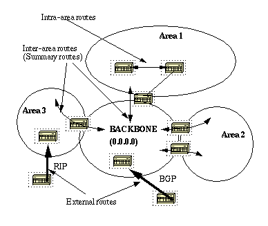
In this diagram, all areas are directly connected to the backbone. In the rare situations where a new area is introduced that cannot have a direct physical access to the backbone, a virtual link has to be configured.
Virtual links are discussed in the next section. Note the different types of routing information. Routes that are generated from within an area (the destination belongs to the area) are called intra-area routes.
These routes are normally represented by the letter O in the IP routing table. Routes that originate from other areas are called inter-area or Summary routes.
The notation for these routes is O IA in the IP routing table. Routes that originate from other routing protocols (or different OSPF processes) and that are injected into OSPF via redistribution are called external routes.
These routes are represented by O E2 or O E1 in the IP routing table. Multiple routes to the same destination are preferred in this order: intra-area, inter-area, external E1, external E2. External types E1 and E2 are explained later.
Virtual Links
Virtual links are used for two purposes:
- To an area that does not have a physical connection to the backbone
- To patch the backbone in case discontinuity of area 0 occurs.
Areas Not Physically Connected to Area 0
As mentioned earlier, area 0 has to be at the center of all other areas. In some rare case where it is impossible to have an area physically connected to the backbone, a virtual link is used.
The virtual link provides the disconnected area a logical path to the backbone. The virtual link has to be established between two ABRs that have a common area, with one ABR connected to the backbone.
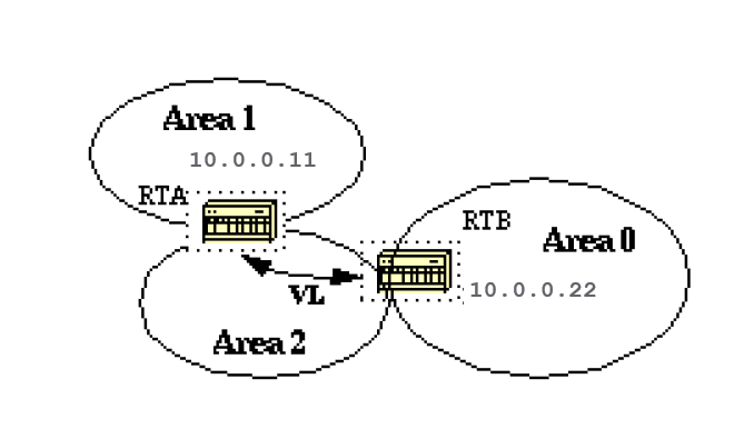
In this example, area 1 does not have a direct physical connection into area 0. A virtual link has to be configured between RTA and RTB. Area 2 is to be used as a transit area and RTB is the entry point into area 0.
In this way RTA and area 1 has a logical connection to the backbone. In order to configure a virtual link, use the area <area-id> virtual-link <RID> router OSPF sub-command on both RTA and RTB, where area-id is the transit area.
In the diagram, this is area 2. The RID is the router-id. The OSPF router-id is usually the highest IP address on the box, or the highest loopback address if one exists.
The router-id is only calculated at boot time. To find the router-id, use the show ip ospf interface command.
Consider that 10.0.0.11 and 10.0.0.22 are the respective RIDs of RTA and RTB, the OSPF configuration for both routers would be:
RTA#
router ospf 10
area 2 virtual-link 10.0.0.22


RTB#
router ospf 10
area 2 virtual-link 10.0.0.11
the Backbone
OSPF allows for discontinuous parts of the backbone to link through a virtual link. In some cases, different area 0s need to be linked together.
This can occur if, for example, a company tries to merge two separate OSPF networks into one network with a common area 0. In other instances, virtual-links are added for redundancy in case some router failure causes the backbone to be split into two.
A virtual link can be configured between separate ABRs that touch area 0 from each side and share a common area (illustrated here).
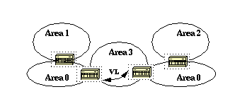
In this diagram, two area 0s are linked together via a virtual link. In case a common area does not exist, an additional area, such as area 3, could be created to become the transit area.
In case any area which is different than the backbone becomes partitioned, the backbone takes care of the partition effort without the use of any virtual links.
One part of the partioned area is known to the other part via inter-area routes rather than intra-area routes.
Neighbors
Routers that share a common segment become neighbors on that segment. Neighbors are elected via the Hello protocol. Hello packets are sent periodically out of each interface through IP multicast (Appendix B).
Routers become neighbors as soon as they see themselves listed in the neighbor Hello packet. This way, a two way communication is guaranteed. Neighbor negotiation applies to the primary address only.
Secondary addresses can be configured on an interface with a restriction that they have to belong to the same area as the primary address.
Two routers do not become neighbors unless they agree with this criteria.
Area-id:Two routers which have a common segment; their interfaces have to belong to the same area on that segment. The interfaces must belong to the same subnet and have a similar mask.Authentication:OSPF allows for the configuration of a password for a specific area. Routers that want to become neighbors have to exchange the same password on a particular segment.Hello and Dead Intervals:OSPF exchangesHellopackets on each segment. This is a form of keepalive used by routers in order to acknowledge their existence on a segment and in order to elect a designated router (DR) on multiaccess segments.
The Hello interval specifies the length of time, in seconds, between the Hello packets that a router sends on an OSPF interface.
The dead interval is the number of seconds that a router Hello packets have not been seen before its neighbors declare the OSPF router down.
- OSPF requires these intervals to be exactly the same between two neighbors. If any of these intervals are different, these routers do not become neighbors on a particular segment. The router interface commands used to set these timers are:
ip ospf hello-interval secondsandip ospf dead-interval seconds. Stub area flag:Two routers have to also agree on the stub area flag in theHellopackets in order to become neighbors. Stub areas are discussed in a later section. Consider that definition of stub areas affect the neighbor election process.
Adjacencies
Adjacency is the next step after the neighbor process. Adjacent routers are routers that go beyond the simple Hello exchange and proceed into the database exchange process.
In order to minimize the amount of information exchange on a particular segment, OSPF elects one router to be a designated router (DR), and one router to be a backup designated router (BDR), on each multi-access segment.
The BDR is elected as a backup mechanism in case the DR goes down. The idea behind this is that routers have a central point of contact for information exchange.
Rather than exchange updates with every other router on the segment, every router exchanges information with the DR and BDR.
The DR and BDR relay the information to everybo creationdy else. In mathematical terms, this cuts the information exchange from O(n*n) to O(n) where n is the number of routers on a multi-access segment.
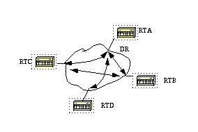
This router model illustrates the DR and BDR:
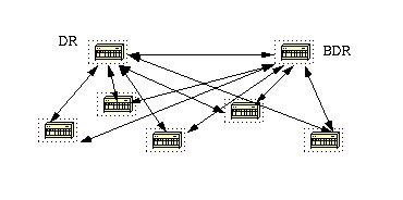
In this diagram, all routers share a common multi-access segment. Due to the exchange of Hello packets, one router is elected DR and another is elected BDR.
Each router on the segment (which already became a neighbor) tries to establish an adjacency with the DR and BDR.
DR Election
DR and BDR election is done via the Hello protocol. Hello packets are exchanged via IP multicast packets (Appendix B) on each segment.
The router with the highest OSPF priority on a segment becomes the DR for that segment. The same process is repeated for the BDR. In case of a tie, the router with the highest RID prevails.
The default for the interface OSPF priority is one. Remember that the DR and BDR concepts are per multiaccess segment. The OSPF priority value on an interface is done with the ip ospf priority <value> interface command.
A priority value of zero indicates an interface which is not to be elected as DR or BDR. The state of the interface with priority zero is DROTHER. This illustrates the DR election:
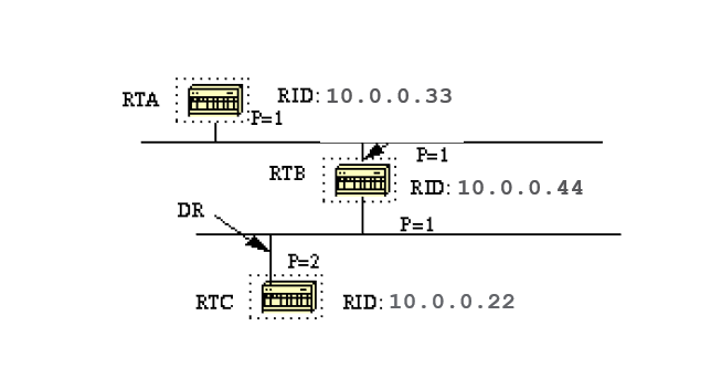
In this diagram, RTA and RTB have the same interface priority but RTB has a higher RID. RTB would be DR on that segment. RTC has a higher priority than RTB. RTC is DR on that segment.
Build the Adjacency
The adjacency build process takes effect after multiple stages have been fulfilled. Routers that become adjacent have the exact link-state database.
Here is a summary of states which an interface passes through before it becomes adjacent to another router:
- Down: No information has been received from anybody on the segment.
- Attempt: On non-broadcast multi-access clouds such as Frame Relay and X.25, this state indicates that no recent information has been received from the neighbor. To contact the neighbor, send Hello packets at the reduced rate Poll Interval .
- Init: The interface has detected a Hello packet from a neighbor but bi-directional communication has not yet been established.
- Two-way: There is bi-directional communication with a neighbor. The router has seen itself in the Hello packets from a neighbor. At the end of this stage the DR and BDR election would have been done. At the end of the 2-way stage, routers decides whether to proceed in an adjacency build. The decision is based on whether one of the routers is a DR or BDR or the link is a point-to-point or a virtual link.
- Exstart: Routers try to establish the initial sequence number to be used in the information exchange packets. The sequence number insures that routers always get the most recent information. One router becomes the primary and the other becomes secondary. The primary router polls the secondary for information.
- Exchange: Routers describe their entire link-state database through sent database description packets. At this state, packets could be flooded to other interfaces on the router.
- Load: At this state, routers finalize the information exchange. Routers have built a link-state request list and a link-state retransmission list. Any information that looks incomplete or outdated are put on the request list. Updates are put on the retransmission list until acknowledged.
- Full: At this state, the adjacency is complete. The neighbor routers are fully adjacent. Adjacent routers have a similar link-state database.
Here is an example:
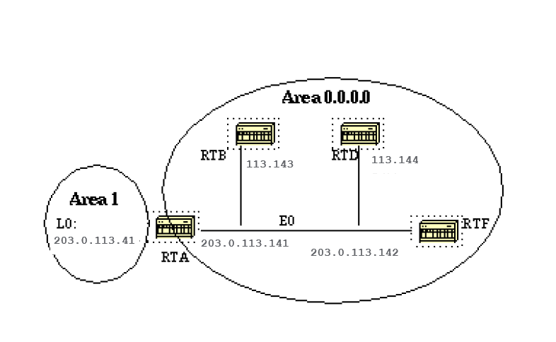
RTA, RTB, RTD, and RTF share a common segment (E0) in area 0.0.0.0. These are the configurations of RTA and RTF. RTB and RTD must have a similar configuration to RTF and are not included.
RTA#
hostname RTA

interface Loopback0
 ip address 203.0.113.41 255.255.255.0

interface Ethernet0
 ip address 203.0.113.141 255.255.255.0

router ospf 10
 network 203.0.113.41 0.0.0.0 area 1
 network 203.0.113.100 0.0.255.255 area 0.0.0.0

RTF#
hostname RTF
interface Ethernet0
 ip address 203.0.113.142 255.255.255.0

router ospf 10
 network 203.0.113.100 0.0.255.255 area 0.0.0.0
This is a simple example that demonstrates a couple of commands that are very useful in debugging OSPF networks.
show ip ospf interface <interface>
This command is a quick check to determine if all of the interfaces belong to the areas they are supposed to be in. The sequence in which the OSPF network commands are listed is very important.
In RTA configuration, if the «network 203.0.113.100 0.0.255.255 area 0.0.0.0» statement was put before the «network 203.0.113.41 0.0.0.0 area 1» statement, all of the interfaces would be in area 0, which is incorrect because the loopback is in area 1.
Here is the command output on RTA, RTF, RTB, and RTD:
RTA#show ip ospf interface e0
Ethernet0 is up, line protocol is up
  Internet Address 203.0.113.141 255.255.255.0, Area 0.0.0.0
  Process ID 10, Router ID 203.0.113.41, Network Type BROADCAST, Cost:
10
  Transmit Delay is 1 sec, State BDR, Priority 1
  Designated Router (ID) 203.0.113.151, Interface address 203.0.113.142
  Backup Designated router (ID) 203.0.113.41, Interface address
203.0.113.141
  Timer intervals configured, Hello 10, Dead 40, Wait 40, Retransmit 5
    Hello due in 0:00:02
  Neighbor Count is 3, Adjacent neighbor count is 3
    Adjacent with neighbor 203.0.113.151  (Designated Router)
Loopback0 is up, line protocol is up
  Internet Address 203.0.113.41 255.255.255.255, Area 1
  Process ID 10, Router ID 203.0.113.41, Network Type LOOPBACK, Cost: 1
  Loopback interface is treated as a stub Host


RTF#show ip ospf interface e0
Ethernet0 is up, line protocol is up
  Internet Address 203.0.113.142 255.255.255.0, Area 0.0.0.0
  Process ID 10, Router ID 203.0.113.151, Network Type BROADCAST, Cost: 10
  Transmit Delay is 1 sec, State DR, Priority 1
  Designated Router (ID) 203.0.113.151, Interface address 203.0.113.142
  Backup Designated router (ID) 203.0.113.41, Interface address
203.0.113.141
  Timer intervals configured, Hello 10, Dead 40, Wait 40, Retransmit 5
    Hello due in 0:00:08
  Neighbor Count is 3, Adjacent neighbor count is 3
    Adjacent with neighbor 203.0.113.41  (Backup Designated Router)


RTD#show ip ospf interface e0
Ethernet0 is up, line protocol is up
  Internet Address 203.0.113.144 255.255.255.0, Area 0.0.0.0
  Process ID 10, Router ID 192.0.2.174, Network Type BROADCAST, Cost:
10
  Transmit Delay is 1 sec, State DROTHER, Priority 1
  Designated Router (ID) 203.0.113.151, Interface address 203.0.113.142
  Backup Designated router (ID) 203.0.113.41, Interface address
203.0.113.141
  Timer intervals configured, Hello 10, Dead 40, Wait 40, Retransmit 5
    Hello due in 0:00:03
  Neighbor Count is 3, Adjacent neighbor count is 2
    Adjacent with neighbor 203.0.113.151  (Designated Router)
    Adjacent with neighbor 203.0.113.41  (Backup Designated Router)


RTB#show ip ospf interface e0
Ethernet0 is up, line protocol is up
  Internet Address 203.0.113.143 255.255.255.0, Area 0.0.0.0
  Process ID 10, Router ID 203.0.113.121, Network Type BROADCAST, Cost: 10
  Transmit Delay is 1 sec, State DROTHER, Priority 1
  Designated Router (ID) 203.0.113.151, Interface address 203.0.113.142
  Backup Designated router (ID) 203.0.113.41, Interface address
203.0.113.141
  Timer intervals configured, Hello 10, Dead 40, Wait 40, Retransmit 5
    Hello due in 0:00:03
  Neighbor Count is 3, Adjacent neighbor count is 2
    Adjacent with neighbor 203.0.113.151  (Designated Router)
    Adjacent with neighbor 203.0.113.41  (Backup Designated Router)
This output shows very important information. At RTA output, Ethernet0 is in area 0.0.0.0. The process ID is 10 (router ospf 10) and the router ID is 203.0.113.41.
Remember that the RID is the highest IP address on the box or the loopback interface, calculated at boot time or whenever the OSPF process is restarted.
The state of the interface is BDR. Since all routers have the same OSPF priority on Ethernet 0 (default is 1), the RTF interface was elected as DR because of the higher RID.
In the same way, RTA was elected as BDR. RTD and RTB are neither a DR or BDR and their state is DROTHER.
Take notice of the neighbor count and the adjacent count. RTD has three neighbors and is adjacent to two of them, the DR and the BDR. RTF has three neighbors and is adjacent to all of them because it is the DR.
The information about the network type is important and determines the state of the interface. On broadcast networks such as Ethernet, the election of the DR and BDR are irrelevant to the end user.
It does not matter who the DR or BDR are. In other cases, such as NBMA media such as Frame Relay and X.25, this becomes very important for OSPF to function correctly.
With the introduction of point-to-point and point-to-multipoint subinterfaces, DR election is no longer an issue. OSPF over NBMA is discussed in the next section.
Another command we need to look at is:
show ip ospf neighbor
Let us look at the RTD output:
RTD#show ip ospf neighbor

Neighbor ID    Pri State         Dead Time  Address      Interface

203.0.113.121    1  2WAY/DROTHER  0:00:37   203.0.113.143  Ethernet0
203.0.113.151    1  FULL/DR       0:00:36   203.0.113.142  Ethernet0
203.0.113.41   1  FULL/BDR      0:00:34   203.0.113.141  Ethernet0
The show ip ospf neighbor command shows the state of all the neighbors on a particular segment. Do not be alarmed if the Neighbor ID does not belong to the segment that you look at.
In our case 203.0.113.121 and 203.0.113.151 are not on Ethernet0. The Neighbor ID is actually the RID which could be any IP address on the box.
RTD and RTB are just neighbors, that is why the state is 2WAY/DROTHER. RTD is adjacent to RTA and RTF and the state is FULL/DR and FULL/BDR.
Adjacencies on Point-to-Point Interfaces
OSPF always forms an adjacency with the neighbor on the other side of a point-to-point interface such as point-to-point serial lines. There is no concept of DR or BDR. The state of the serial interfaces is point to point.
Adjacencies on Non-Broadcast Multi-Access (NBMA) Networks
Special care must be taken with configuration of OSPF over multi-access non-broadcast medias such as Frame Relay, X.25, ATM. The protocol considers these media like any other broadcast media such as Ethernet.
NBMA clouds are usually built in a hub and spoke topology. PVCs or SVCs are laid out in a partial mesh and the physical topology does not provide the multi access that OSPF can detect.
The selection of the DR becomes an issue because the DR and BDR need to have full physical connectivity with all routers that exist on the cloud.
Because of the lack of broadcast capabilities, the DR and BDR need to have a static list of all other routers attached to the cloud.
This is achieved with the neighbor ip-address [priority number] [poll-interval seconds] command, where the «ip-address» and «priority» are the IP address and the OSPF priority given to the neighbor.
A neighbor with priority 0 is considered ineligible for DR election. The «poll-interval» is the amount of time an NBMA interface waits before the poll (a sent Hello) to a presumably dead neighbor.
The neighbor command applies to routers with DR- or BDR-potential (interface priority not equal to 0). This shows a network diagram where DR selection is very important:
In this diagram, it is essential for the RTA interface to the cloud to be elected DR. This is because RTA is the only router that has full connectivity to other routers.
The election of the DR could be influenced by the ospf priority parameter on the interfaces. Routers that do not need to become DRs or BDRs have a priority of 0 other routers could have a lower priority.
The neighbor command is not covered in depth in this document and becomes obsolete through new interface Network Type irrespective of the underlying physical media. This is explained in the next section.
Avoid DRs and neighbor Command on NBMA
Different methods can be used to avoid the complications of static neighbor configuration and specific routers which become DRs or BDRs on the non-broadcast cloud.
To specify which method to use is influenced by whether we are start the network from the start or if we rectify a design which already exists.
Point-to-Point Subinterfaces
A subinterface is a logical way to define an interface. The same physical interface can be split into multiple logical interfaces, with each subinterface defined as point-to-point.
This was originally created in order to better handle issues caused by split horizon over NBMA and vector based routing protocols.
A point-to-point subinterface has the properties of any physical point-to-point interface. As far as OSPF is concerned, an adjacency is always formed over a point-to-point subinterface with no DR or BDR election.
This is an illustration of point-to-point subinterfaces:
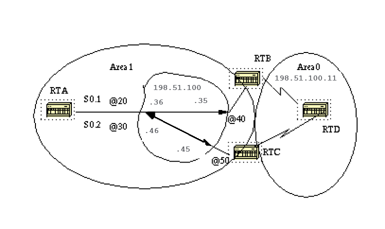
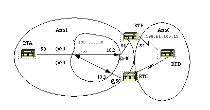
In this diagram, on RTA, we can split Serial 0 into two point-to-point subinterfaces, S0.1 and S0.2. This way, OSPF considers the cloud as a set of point-to-point links rather than one multi-access network.
The only drawback for the point-to-point is that each segment belongs to a different subnet. This is unacceptable because some administrators have already assigned one IP subnet for the whole cloud.
Another workaround is to use IP unnumbered interfaces on the cloud. This is also a problem for administrators who manage the WAN based on IP addresses of the serial lines. This is a typical configuration for RTA and RTB:
RTA#

interface Serial 0
 no ip address
 encapsulation frame-relay

interface Serial0.1 point-to-point
 ip address 198.51.100.36 255.255.252.0
 frame-relay interface-dlci 20

interface Serial0.2 point-to-point
 ip address 198.51.100.46 255.255.252.0
 frame-relay interface-dlci 30

router ospf 10
network 198.51.100.1 0.0.255.255 area 1

RTB#

interface Serial 0
 no ip address
 encapsulation frame-relay

interface Serial0.1 point-to-point
 ip address 198.51.100.35 255.255.252.0
 frame-relay interface-dlci 40

interface Serial1
 ip address 198.51.100.11 255.255.255.0

router ospf 10
network 198.51.100.1 0.0.255.255 area 1
network 198.51.100.10 0.0.255.255 area 0
Select Interface Network Types
The command used to set the network type of an OSPF interface is:
ip ospf network {broadcast | non-broadcast | point-to-multipoint}
Point-to-Multipoint Interfaces
An OSPF point-to-multipoint interface is defined as a numbered point-to-point interface with one or more neighbors. This concept takes the previously discussed point-to-point concept one step further.
Administrators do not have to worry about multiple subnets for each point-to-point link. The cloud is configured as one subnet.
This works well for those who migrate into the point-to-point concept with no change in IP address on the cloud. Also, they can disregard DRs and neighbor statements.
OSPF point-to-multipoint works through the exchange of additional link-state updates that contain a number of information elements that describe connectivity to the neighbor routers.
RTA#

interface Loopback0
 ip address 203.0.113.101 255.255.255.0

interface Serial0
 ip address 198.51.100.101 255.255.255.0
 encapsulation frame-relay
 ip ospf network point-to-multipoint

router ospf 10
network 198.51.100.1 0.0.255.255 area 1

RTB#

interface Serial0
 ip address 198.51.100.102 255.255.255.0
 encapsulation frame-relay
 ip ospf network point-to-multipoint

interface Serial1
 ip address 198.51.100.11 255.255.255.0

router ospf 10
network 198.51.100.1 0.0.255.255 area 1
network 198.51.100.10 0.0.255.255 area 0
Note that no static frame relay map statements were configured; this is because Inverse ARP takes care of the DLCI to IP address mapping. Let us look at some of show ip ospf interface and show ip ospf route outputs:
RTA#show ip ospf interface s0
Serial0 is up, line protocol is up
  Internet Address 198.51.100.101 255.255.255.0, Area 0
  Process ID 10, Router ID 203.0.113.101, Network Type
POINT_TO_MULTIPOINT, Cost: 64
  Transmit Delay is 1 sec, State POINT_TO_MULTIPOINT,
  Timer intervals configured, Hello 30, Dead 120, Wait 120, Retransmit 5
    Hello due in 0:00:04
  Neighbor Count is 2, Adjacent neighbor count is 2
    Adjacent with neighbor 198.51.100.174
    Adjacent with neighbor 198.51.100.130

RTA#show ip ospf neighbor

Neighbor ID     Pri   State           Dead Time   Address         Interface
198.51.100.103      1   FULL/  -        0:01:35     198.51.100.103    Serial0
198.51.100.102      1   FULL/  -        0:01:44     198.51.100.102    Serial0

RTB#show ip ospf interface s0

Serial0 is up, line protocol is up
  Internet Address 198.51.100.102 255.255.255.0, Area 0
  Process ID 10, Router ID 198.51.100.102, Network Type
POINT_TO_MULTIPOINT, Cost: 64
  Transmit Delay is 1 sec, State POINT_TO_MULTIPOINT,
  Timer intervals configured, Hello 30, Dead 120, Wait 120, Retransmit 5
    Hello due in 0:00:14
  Neighbor Count is 1, Adjacent neighbor count is 1
    Adjacent with neighbor 203.0.113.101

RTB#show ip ospf neighbor

Neighbor ID     Pri   State           Dead Time   Address         Interface
203.0.113.101      1   FULL/  -        0:01:52     198.51.100.101    Serial0
The only drawback for point-to-multipoint is that it generates multiple Hosts routes (routes with mask 255.255.255.255) for all the neighbors. Note the Host routes in the IP routing table for RTB:
RTB#show ip route
 Codes: C - connected, S - static, I - IGRP, R - RIP, M - mobile, B - BGP
        D - EIGRP, EX - EIGRP external, O - OSPF, IA - OSPF inter area
        E1 - OSPF external type 1, E2 - OSPF external type 2, E - EGP
        i - IS-IS, L1 - IS-IS level-1, L2 - IS-IS level-2, * - candidate default

 Gateway of last resort is not set

      203.0.113.210 255.255.255.255 is subnetted, 1 subnets
 O       203.0.113.101 [110/65] via 198.51.100.101,  Serial0
         198.51.100.1 is variably subnetted, 3 subnets, 2 masks
 O    198.51.100.103 255.255.255.255
            [110/128] via 198.51.100.101, 00:00:00, Serial0
 O    198.51.100.101 255.255.255.255
            [110/64] via 198.51.100.101, 00:00:00, Serial0
 C       198.51.100.100 255.255.255.0 is directly connected, Serial0
      172.16.0.0 255.255.255.0 is subnetted, 1 subnets
 C       172.16.0.1 is directly connected, Serial1

 RTC#show ip route

      203.0.113.210 255.255.255.255 is subnetted, 1 subnets
 O       203.0.113.101 [110/65] via 198.51.100.101, Serial1
      198.51.100.1 is variably subnetted, 4 subnets, 2 masks
 O       198.51.100.102 255.255.255.255 [110/128] via 198.51.100.101,Serial1
 O       198.51.100.101 255.255.255.255 [110/64] via 198.51.100.101, Serial1
 C       198.51.100.100 255.255.255.0 is directly connected, Serial1
      172.16.0.0 255.255.255.0 is subnetted, 1 subnets
 O       172.16.0.1 [110/192] via 198.51.100.101, 00:14:29, Serial1
Note that in the RTC IP routing table, network 172.16.0.1 is reachable via next hop 198.51.100.101 and not via 198.51.100.102, normally seen over Frame Relay clouds which share the same subnet.
This is one advantage of the point-to-multipoint configuration because you do not need static mapping on RTC to reach next hop 198.51.100.102.
Broadcast Interfaces
This approach is a workaround for the neighbor command which statically lists all current neighbors. The interface is logically set to broadcast and behaves as if the router were connected to a LAN.
DR and BDR election are performed so assure that either a full mesh topology or a static selection of the DR based on the interface priority. The command that sets the interface to broadcast is:
ip ospf network broadcast
OSPF and Route Summarization
To summarize is to consolidate multiple routes into one single advertisement. This is normally done at the boundaries of Area Border Routers (ABRs).
Although summarization is configured between any two areas, it is better to summarize in the direction of the backbone. This way the backbone receives all the aggregate addresses and in turn injects them, already summarized, into other areas.
There are two types of summarization:
- Inter-area route summarization
- External route summarization
Inter-Area Route Summarization
Inter-area route summarization is done on ABRs and it applies to routes from within the AS. It does not apply to external routes injected into OSPF via redistribution.
In order to take advantage of summarization, network numbers in areas must be assigned in a contiguous way to lump these addresses into one range.
To specify an address range, perform this task in router configuration mode:
area area-id range address mask
Where the area-id is the area which contains networks to be summarized. The «address» and «mask» specifies the range of addresses to be summarized in one range. This is an example of summarization:
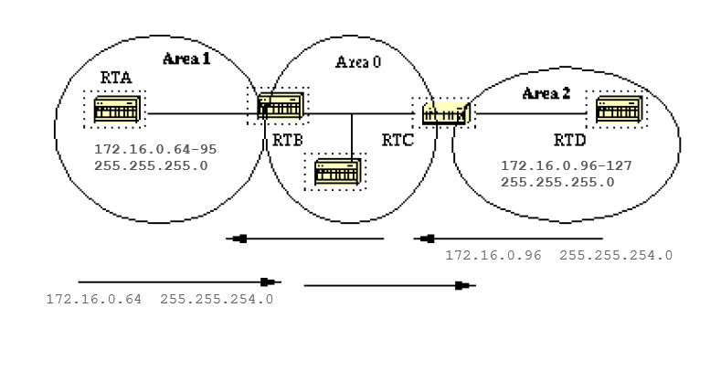
In this diagram, RTB isummarizes the range of subnets from 172.16.0.64 to 172.16.0.95 into one range: 172.16.0.64 255.255.224.0. To achieve this, mask the first three left most bits of 64 with a mask of 255.255.224.0.
In the same way, RTC generates the summary address 172.16.0.96 255.255.224.0 into the backbone. Note that this summarization was successful because we have two distinct ranges of subnets, 64-95 and 96-127.
It is difficult to summarize if the subnets between area 1 and area 2 overlapped. The backbone area would receive summary ranges that overlap and routers in the middle would not know where to send the traffic based on the summary address.
This is the relative configuration of RTB:
RTB#
 router ospf 100
 area 1 range 172.16.0.64 255.255.224.0
Prior to Cisco IOS® Software Release 12.1(6), it was recommended to manually configure, on the ABR, a discard static route for the summary address to prevent possible routing loops. For the summary route shown, use this command:
ip route 172.16.0.64 255.255.224.0 null0
In Cisco IOS® 12.1(6) and higher, the discard route is automatically generated by default. To discard route, configure commands under router ospf:
- Either
[no] discard-route internal - Or
[no] discard-route external
Note about summary address metric calculation: RFC 1583 called to calculate the metric for summary routes based on the minimum metric of the component paths available.
RFC 2178 (now obsoleted by RFC 2328) changed the specified method to calculate metrics for summary routes so the component of the summary with the maximum (or largest) cost would determine the cost of the summary.
Prior to Cisco IOS® 12.0, Cisco was compliant with the then-current RFC 1583. As of Cisco IOS® 12.0, Cisco changed the behavior of OSPF to be compliant with the new standard, RFC 2328.
This situation created the possibility of sub-optimal routing if all of the ABRs in an area were not upgraded to the new code at the same time.
In order to address this potential problem, a command has been added to the OSPF configuration of Cisco IOS® that allows you to selectively disable compatibility with RFC 2328.
The new configuration command is under router ospf, and has the syntax:
[no] compatible rfc1583
The default parameter is compatible with RFC 1583. This command is available in these versions of Cisco IOS®:
- 12.1(03)DC
- 12.1(03)DB
- 12.001(001.003) — 12.1 Mainline
- 12.1(01.03)T — 12.1 T-Train
- 12.000(010.004) — 12.0 Mainline
- 12.1(01.03)E — 12.1 E-Train
- 12.1(01.03)EC
- 12.0(10.05)W05(18.00.10)
- 12.0(10.05)SC
External Route Summarization
External route summarization is specific to external routes that are injected into OSPF via redistribution. Also, make sure that external ranges that are summarized are contiguous.
Summarization of overlapped ranges from two different routers could cause packets to be sent to the wrong destination. Summarization is done via the router ospf subcommand:
summary-address ip-address mask
This command is effective only on ASBR redistribution into OSPF.
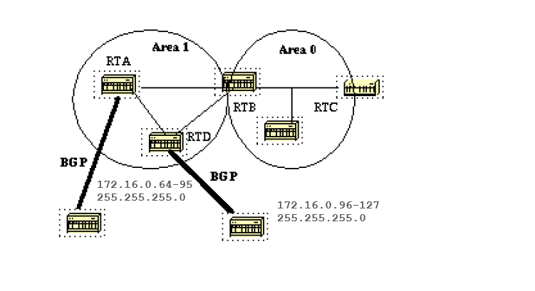
In this diagram, RTA and RTD inject external routes into OSPF by redistribution. RTA injects subnets in the range 128.213.64-95 and RTD injects subnets in the range 128.213.96-127. To summarize the subnets into one range on each router:
RTA#
 router ospf 100
 summary-address 172.16.0.64 255.255.224.0
 redistribute bgp 50 metric 1000 subnets

 RTD#
 router ospf 100
 summary-address 172.16.0.96 255.255.224.0
 redistribute bgp 20 metric 1000 subnets
This causes RTA to generate one external route 172.16.0.64 255.255.224.0 and causes RTD to generate 172.16.0.96 255.255.224.0.
Note that the summary-address command has no effect if used on RTB because RTB does not perform the redistribution into OSPF.
Stub Areas
OSPF allows certain areas to be configured as stub areas. External networks, such as those redistributed from other protocols into OSPF, are not allowed to be flooded into a stub area.
Routing from these areas to the outside world is based on a default route. Stub area configuration reduces the topological database size inside an area and reduces the memory requirements of routers inside that area.
An area could be qualified a stub when there is a single exit point from that area or if routing to outside of the area does not have to take an optimal path.
The latter description is an indication that a stub area that has multiple exit points also has one or more area border routers which inject a default into that area.
Routing to the outside world could take a sub-optimal path to the destination out of the area via an exit point which is farther to the destination than other exit points.
Other stub area restrictions are that a stub area cannot be used as a transit area for virtual links. Also, an ASBR cannot be internal to a stub area.
These restrictions are made because a stub area is mainly configured not to carry external routes and any of these situations cause external links to be injected in that area. The backbone cannot be configured as stub.
All OSPF routers inside a stub area have to be configured as stub routers. When an area is configured as stub, all interfaces that belong to that area exchange Hello packets with a flag that indicates that the interface is stub.
Actually this is just a bit in the Hello packet (E bit) that gets set to 0. All routers that have a common segment have to agree on that flag. Otherwise, then they do not become neighbors and routing does not take effect.
An extension to stub areas is called totally stubby areas. Cisco indicates this with the addition of a no-summary keyword to the stub area configuration.
A totally stubby area is one that blocks external routes and summary routes (inter-area routes) from entrance into the area.
This way, intra-area routes and the default of 0.0.0.0 are the only routes injected into that area.
- The command that configures an area as stub is:
area <area-id> stub [no-summary] - The command that configures a default-cost into an area is:
area area-id default-cost cost
If the cost is not set with that command, a cost of 1 is advertised by the ABR.
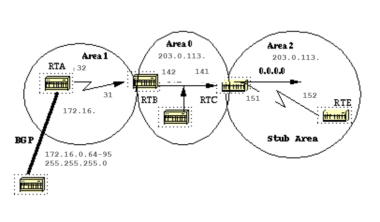
Assume that area 2 is to be configured as a stub area. This example shows the routing table of RTE before and after area 2 stub configuration.
RTC#

 interface Ethernet 0
  ip address 203.0.113.141 255.255.255.0

 interface Serial1
  ip address 203.0.113.151 255.255.255.252

 router ospf 10
  network 203.0.113.150 0.0.0.255 area 2
  network 203.0.113.140 0.0.0.255 area 0
 RTE#show ip route
 Codes: C - connected, S - static, I - IGRP, R - RIP, M - mobile, B - BGP
        D - EIGRP, EX - EIGRP external, O - OSPF, IA - OSPF inter area
        E1 - OSPF external type 1, E2 - OSPF external type 2, E - EGP
        i - IS-IS, L1 - IS-IS level-1, L2 - IS-IS level-2, * - candidate default

 Gateway of last resort is not set

      203.0.113.150 255.255.255.252 is subnetted, 1 subnets
 C       203.0.113.150 is directly connected, Serial0
 O IA 203.0.113.140 [110/74] via 203.0.113.151, 00:06:31, Serial0
      198.51.100.1 is variably subnetted, 2 subnets, 2 masks
 O E2    172.16.0.64 255.255.192.0
            [110/10] via 203.0.113.151, 00:00:29, Serial0
 O IA    172.16.0.63 255.255.255.252
            [110/84] via 203.0.113.151, 00:03:57, Serial0
      172.16.0.108 255.255.255.240 is subnetted, 1 subnets
 O       172.16.0.208 [110/74] via 203.0.113.151, 00:00:10, Serial0
RTE has learned the inter-area routes (O IA) 203.0.113.140 and 172.16.0.63 and it has learned the intra-area route (O) 172.16.0.208 and the external route (O E2) 172.16.0.64.
To configure area 2 as stub:
RTC#

 interface Ethernet 0
  ip address 203.0.113.141 255.255.255.0

 interface Serial1
  ip address 203.0.113.151 255.255.255.252

 router ospf 10
  network 203.0.113.150 0.0.0.255 area 2
  network 203.0.113.140 0.0.0.255 area 0
  area 2 stub

 RTE#

 interface Serial1
  ip address 203.0.113.152 255.255.255.252
 router ospf 10
 network 203.0.113.150 0.0.0.255 area 2
  area 2 stub
Note that the stub command is configured on RTE also, otherwise RTE never becomes a neighbor to RTC. The default cost was not set, so RTC advertises 0.0.0.0 to RTE with a metric of 1.
RTE#show ip route
 Codes: C - connected, S - static, I - IGRP, R - RIP, M - mobile, B - BGP
        D - EIGRP, EX - EIGRP external, O - OSPF, IA - OSPF inter area
        E1 - OSPF external type 1, E2 - OSPF external type 2, E - EGP
        i - IS-IS, L1 - IS-IS level-1, L2 - IS-IS level-2, * - candidate default

 Gateway of last resort is 203.0.113.151 to network 0.0.0.0

      203.0.113.150 255.255.255.252 is subnetted, 1 subnets
 C       203.0.113.150 is directly connected, Serial0
 O IA 203.0.113.140 [110/74] via 203.0.113.151, 00:26:58, Serial0
      198.51.100.1 255.255.255.252 is subnetted, 1 subnets
 O IA    172.16.0.63 [110/84] via 203.0.113.151, 00:26:59, Serial0
      172.16.0.108 255.255.255.240 is subnetted, 1 subnets
 O       172.16.0.208 [110/74] via 203.0.113.151, 00:26:59, Serial0
 O*IA 0.0.0.0 0.0.0.0 [110/65] via 203.0.113.151, 00:26:59, Serial0
Note that all the routes show up except the external routes which were replaced by a default route of 0.0.0.0. The cost of the route happened to be 65 (64 for a T1 line + 1 advertised by RTC).
We now configure area 2 to be totally stubby, and change the default cost of 0.0.0.0 to 10.
RTC#

 interface Ethernet 0
  ip address 203.0.113.141 255.255.255.0

 interface Serial1
  ip address 203.0.113.151 255.255.255.252

 router ospf 10
  network 203.0.113.150 0.0.0.255 area 2
  network 203.0.113.140 0.0.0.255 area 0
  area 2 stub no-summary
  area 2 default cost 10


 RTE#show ip route

 Codes: C - connected, S - static, I - IGRP, R - RIP, M - mobile, B - BGP
        D - EIGRP, EX - EIGRP external, O - OSPF, IA - OSPF inter area
        E1 - OSPF external type 1, E2 - OSPF external type 2, E - EGP
        i - IS-IS, L1 - IS-IS level-1, L2 - IS-IS level-2, * - candidate default

 Gateway of last resort is not set

      203.0.113.150 255.255.255.252 is subnetted, 1 subnets
 C       203.0.113.150 is directly connected, Serial0
      172.16.0.108 255.255.255.240 is subnetted, 1 subnets
 O       172.16.0.208 [110/74] via 203.0.113.151, 00:31:27, Serial0
 O*IA 0.0.0.0 0.0.0.0 [110/74] via 203.0.113.151, 00:00:00, Serial0
Note that the only routes that show up are the intra-area routes (O) and the default-route 0.0.0.0. The external and inter-area routes have been blocked.
The cost of the default route is now 74 (64 for a T1 line + 10 advertised by RTC). No configuration is needed on RTE in this case.
The area is already stub, and the no-summary command does not affect the Hello packet at all as the stub command does.
Redistribute Routes into OSPF
Redistribute routes into OSPF from other routing protocols or from static causes these routes to become OSPF external routes. To redistribute routes into OSPF, use this command in router configuration mode:
redistribute protocol [process-id] [metric value] [metric-type value] [route-map map-tag] [subnets]
Note: This command must be on one line.
The protocol and process-id are the protocol that we inject into OSPF and its process-id if it exits. The metric is the cost which we are assign to the external route.
If no metric is specified, OSPF puts a default value of 20 when routes are redistributed from all protocols except BGP routes, which get a metric of 1. The metric-type is discussed in the next paragraph.
The route-map is a method used to control the redistribution of routes between routing domains. The format of a route map is:
route-map map-tag [[permit | deny] | [sequence-number]]
With route redistribution into OSPF, only routes that are not subnetted are redistributed if the subnets keyword is not specified.
E1 vs. E2 External Routes
External routes fall under two categories, external type 1 and external type 2. The difference between the two is in the way the cost (metric) of the route is calculated.
The cost of a type 2 route is always the external cost, irrespective of the interior cost to reach that route.
A type 1 cost is the addition of the external cost and the internal cost used to reach that route.
A type 1 route is always preferred over a type 2 route for the same destination.
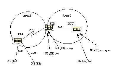
As the this diagram shows, RTA redistributes two external routes into OSPF. N1 and N2 both have an external cost of x. The only difference is that N1 is redistributed into OSPF with a metric-type 1 and N2 is redistributed with a metric-type 2.
If we track the routes as they flow from Area 1 to Area 0, the cost to reach N2 as seen from RTB or RTC is always x. The internal cost along the way is not considered. On the other hand, the cost to reach N1 is incremented by the internal cost. The cost is x+y as seen from RTB and x+y+z as seen from RTC.
If the external routes are both type 2 routes and the external costs to the destination network are equal, then the path with the lowest cost to the ASBR is selected as the best path.
Unless otherwise specified, the default external type given to external routes is type 2.
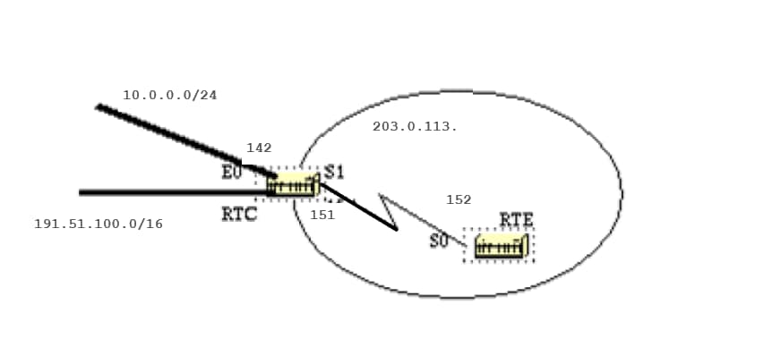
Suppose we added two static routes which point to E0 on RTC: 10.0.0.16 255.255.255.0 (the /24 notation indicates a 24 bit mask which starts from the far left) and 198.51.100.1 255.255.0.0.
This shows the different behaviors when different parameters are used in the redistribute command on RTC:
RTC#
 interface Ethernet0
  ip address 203.0.113.142 255.255.255.0

 interface Serial1
  ip address 203.0.113.151 255.255.255.252

 router ospf 10
  redistribute static
  network 203.0.113.150 0.0.0.255 area 2
  network 203.0.113.140 0.0.0.255 area 0

 ip route 10.0.0.16 255.255.255.0 Ethernet0
 ip route 198.51.100.1 255.255.0.0 Ethernet0

 RTE#

 interface Serial0
  ip address 203.0.113.152 255.255.255.252

 router ospf 10
 network 203.0.113.150 0.0.0.255 area 2
The output of show ip route on RTE:
RTE#show ip route
 Codes: C - connected, S - static, I - IGRP, R - RIP, M - mobile, B - BGP
        D - EIGRP, EX - EIGRP external, O - OSPF, IA - OSPF inter area
        E1 - OSPF external type 1, E2 - OSPF external type 2, E - EGP
        i - IS-IS, L1 - IS-IS level-1, L2 - IS-IS level-2, * - candidate default

 Gateway of last resort is not set

      203.0.113.150 255.255.255.252 is subnetted, 1 subnets
 C       203.0.113.150 is directly connected, Serial0
 O IA 203.0.113.140 [110/74] via 203.0.113.151, 00:02:31, Serial0
 O E2 198.51.100.1 [110/20] via 203.0.113.151, 00:02:32, Serial0
Note that the only external route that has appeared is 198.51.100.1, because we did not use the subnet keyword. Remember that if the subnet keyword is not used, only routes that are not subnetted are redistributed. In our case 10.0.0.16 is a class A route that is subnetted and it did not get redistributed. Since the metric keyword was not used (or a default-metric statement under router OSPF), the cost allocated to the external route is 20 (the default is 1 for BGP).
redistribute static metric 50 subnets

RTE#show ip route
Codes: C - connected, S - static, I - IGRP, R - RIP, M
- mobile, B - BGP
        D - EIGRP, EX - EIGRP external, O - OSPF, IA - OSPF inter area
        E1 - OSPF external type 1, E2 - OSPF external type 2, E - EGP
        i - IS-IS, L1 - IS-IS level-1, L2 - IS-IS level-2, * - candidate default

 Gateway of last resort is not set

      10.0.0.16 255.255.255.0 is subnetted, 1 subnets
 O E2    10.0.0.16 [110/50] via 203.0.113.151, 00:00:02, Serial0
      203.0.113.150 255.255.255.252 is subnetted, 1 subnets
 C       203.0.113.150 is directly connected, Serial0
 O IA 203.0.113.140 [110/74] via 203.0.113.151, 00:00:02, Serial0
 O E2 198.51.100.1 [110/50] via 203.0.113.151, 00:00:02, Serial0
Note that 10.0.0.16 has shown up now and the cost to external routes is 50. Since the external routes are of type 2 (E2), the internal cost has not been added. Suppose now, we change the type to E1:
redistribute static metric 50 metric-type 1 subnets

RTE#show ip route
 Codes: C - connected, S - static, I - IGRP, R - RIP, M - mobile, B - BGP
        D - EIGRP, EX - EIGRP external, O - OSPF, IA - OSPF inter area
        E1 - OSPF external type 1, E2 - OSPF external type 2, E - EGP
        i - IS-IS, L1 - IS-IS level-1, L2 - IS-IS level-2, * - candidate default

 Gateway of last resort is not set

      10.0.0.16 255.255.255.0 is subnetted, 1 subnets
 O E1    10.0.0.16 [110/114] via 203.0.113.151, 00:04:20, Serial0
      203.0.113.150 255.255.255.252 is subnetted, 1 subnets
 C       203.0.113.150 is directly connected, Serial0
 O IA 203.0.113.140 [110/74] via 203.0.113.151, 00:09:41, Serial0
 O E1 198.51.100.1 [110/114] via 203.0.113.151, 00:04:21, Serial0
Note that the type has changed to E1 and the cost has been incremented by the internal cost of S0 which is 64, the total cost is 64+50=114.
Assume that we add a route map to the RTC configuration:
RTC#
 interface Ethernet0
  ip address 203.0.113.142 255.255.255.0

 interface Serial1
  ip address 203.0.113.151 255.255.255.252

 router ospf 10
 redistribute static metric 50 metric-type 1 subnets route-map STOPUPDATE
  network 203.0.113.150 0.0.0.255 area 2
  network 203.0.113.140 0.0.0.255 area 0

 ip route 10.0.0.16 255.255.255.0 Ethernet0
 ip route 198.51.100.1 255.255.0.0 Ethernet0

 access-list 1 permit 198.51.100.1 0.0.255.255

 route-map STOPUPDATE permit 10
  match ip address 1
The route map only permits 198.51.100.1 to be redistributed into OSPF and denies the rest. This is why 10.0.0.16 does not show up in the RTE routing table anymore.
RTE#show ip route
 Codes: C - connected, S - static, I - IGRP, R - RIP, M - mobile, B - BGP
        D - EIGRP, EX - EIGRP external, O - OSPF, IA - OSPF inter area
        E1 - OSPF external type 1, E2 - OSPF external type 2, E - EGP
        i - IS-IS, L1 - IS-IS level-1, L2 - IS-IS level-2, * - candidate default

 Gateway of last resort is not set

      203.0.113.150 255.255.255.252 is subnetted, 1 subnets
 C       203.0.113.150 is directly connected, Serial0
 O IA 203.0.113.140 [110/74] via 203.0.113.151, 00:00:04, Serial0
 O E1 198.51.100.1 [110/114] via 203.0.113.151, 00:00:05, Serial0
Redistribute OSPF into Other Protocols
Use of a Valid Metric
Whenever you redistribute OSPF into other protocols, you have to respect the rules of those protocols. In particular, the metric applied must match the metric used by that protocol.
For example, the RIP metric is a hop count between 1 and 16, where 1 indicates that a network is one hop away and 16 indicates that the network is unreachable. On the other hand IGRP and EIGRP require a metric of the form:
default-metric bandwidth delay reliability loading mtu
VLSM
Another issue to consider is VLSM (Variable Length Subnet Guide)(Appendix C). OSPF can carry multiple subnet information for the same major net, but other protocols such as RIP and IGRP (EIGRP is OK with VLSM) cannot.
If the same major net crosses the boundaries of an OSPF and RIP domain, VLSM information redistributed into RIP or IGRP is lost and static routes have to be configured in the RIP or IGRP domains. This example illustrates this problem.
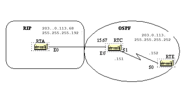
In this diagram, RTE runsOSPF and RTA runs RIP. RTC does the the redistribution between the two protocols. The problem is that the class C network 203.0.113.150 is variably subnetted, it has two different masks 255.255.255.252 and 255.255.255.192.
Here is the configuration and the routing tables of RTE and RTA:
RTA#
 interface Ethernet0
  ip address 203.0.113.68 255.255.255.192
 router rip
  network 203.0.113.150
 RTC#
 interface Ethernet0
  ip address 203.0.113.67 255.255.255.192

 interface Serial1
  ip address 203.0.113.151 255.255.255.252
 router ospf 10
 redistribute rip metric 10 subnets
  network 203.0.113.150 0.0.0.255 area 0
 router rip
  redistribute ospf 10 metric 2
  network 203.0.113.150

 RTE#show ip route
 Codes: C - connected, S - static, I - IGRP, R - RIP, M - mobile, B - BGP
        D - EIGRP, EX - EIGRP external, O - OSPF, IA - OSPF inter area
        E1 - OSPF external type 1, E2 - OSPF external type 2, E - EGP
        i - IS-IS, L1 - IS-IS level-1, L2 - IS-IS level-2, * - candidate default

 Gateway of last resort is not set

      203.0.113.150 is variably subnetted, 2 subnets, 2 masks
 C       203.0.113.150 255.255.255.252 is directly connected, Serial0
 O       203.0.113.64 255.255.255.192
            [110/74] via 203.0.113.151, 00:15:55, Serial0
 RTA#show ip route
 Codes: C - connected, S - static, I - IGRP, R - RIP, M - mobile, B - BGP
        D - EIGRP, EX - EIGRP external, O - OSPF, IA - OSPF inter area
        E1 - OSPF external type 1, E2 - OSPF external type 2, E - EGP
        i - IS-IS, L1 - IS-IS level-1, L2 - IS-IS level-2, * - candidate default

 Gateway of last resort is not set

      203.0.113.150 255.255.255.192 is subnetted, 1 subnets
 C       203.0.113.64 is directly connected, Ethernet0
Note that RTE has recognized that 203.0.113.150 has two subnets while RTA thinks that it has only one subnet (the one configured on the interface).
Information about subnet 203.0.113.150 255.255.255.252 is lost in the RIP domain. In order to reach that subnet, a static route needs to be configured on RTA:
RTA#
 interface Ethernet0
  ip address 203.0.113.68 255.255.255.192
 router rip
  network 203.0.113.150

ip route 203.0.113.150 255.255.255.0 203.0.113.67
This way RTA is able to reach the other subnets.
Mutual Redistribution
Mutual redistribution between protocols must be done very carefully and in a controlled manner. Incorrect configuration could lead to potential looping of routing information.
A rule of thumb for mutual redistribution is not to allow information learned from a protocol to be injected back into the same protocol.
Passive interfaces and distribute lists must be applied on the redistribution routers. To filter information with link-state protocols such as OSPF is a difficult.
Distribute-list out works on the ASBR to filter redistributed routes into other protocols. Distribute-list in works on any router to prevent routes from the routing table, but it does not prevent link-state packets from propagation; downstream routers would still have the routes.
It is better to avoid any OSPF filter as much as possible if filters can be applied on the other protocols to prevent loops.
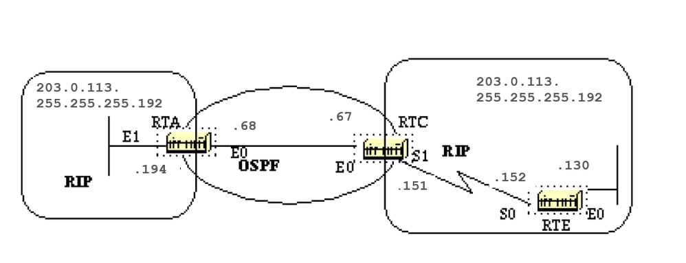
To illustrate, suppose RTA, RTC, and RTE run RIP. RTC and RTA also run OSPF. Both RTC and RTA do redistribution between RIP and OSPF.
If you do not want the RIP from RTE to be injected into the OSPF domain, put a passive interface for RIP on E0 of RTC. However, you have allowed the RIP from RTA to be injected into OSPF. Here is the outcome:
Note: Do not use this configuration.
RTE#
 interface Ethernet0
  ip address 203.0.113.15130 255.255.255.192

 interface Serial0
  ip address 203.0.113.152 255.255.255.192

 router rip
  network 203.0.113.150


RTC#
 interface Ethernet0
  ip address 203.0.113.67 255.255.255.192

 interface Serial1
  ip address 203.0.113.151 255.255.255.192

 router ospf 10
  redistribute rip metric 10 subnets
  network 203.0.113.150 0.0.0.255 area 0

 router rip
  redistribute ospf 10 metric 2
  passive-interface Ethernet0
  network 203.0.113.150


RTA#
interface Ethernet0
 ip address 203.0.113.68 255.255.255.192

router ospf 10
 redistribute rip metric 10 subnets
 network 203.0.113.150 0.0.0.255 area 0


router rip
 redistribute ospf 10 metric 1
 network 203.0.113.150


RTC#show ip route
 Codes: C - connected, S - static, I - IGRP, R - RIP, M - mobile, B - BGP
        D - EIGRP, EX - EIGRP external, O - OSPF, IA - OSPF inter area
        E1 - OSPF external type 1, E2 - OSPF external type 2, E - EGP
        i - IS-IS, L1 - IS-IS level-1, L2 - IS-IS level-2, * - candidate default

 Gateway of last resort is not set

      203.0.113.150 255.255.255.192 is subnetted, 4 subnets
 C       203.0.113.150 is directly connected, Serial1
 C       203.0.113.64 is directly connected, Ethernet0
 R       203.0.113.15128 [120/1] via 203.0.113.68, 00:01:08, Ethernet0
                        [120/1] via 203.0.113.152, 00:00:11, Serial1
 O       203.0.113.15192 [110/20] via 203.0.113.68, 00:21:41, Ethernet0
Note that RTC has two paths to reach 203.0.113.15128 subnet: Serial 1 and Ethernet 0 (E0 is obviously the wrong path). This happened because RTC gave that entry to RTA via OSPF and RTA gave it back via RIP because RTA did not learn it via RIP.
This example is a very small scale of loops that can occur because of an incorrect configuration. In large networks this situation gets even more aggravated.
In order to fix the situation in our example, do not send RIP on RTA Ethernet 0 via a passive interface. This is not suitable in case some routers on the Ethernet are RIP only routers.
In this case, you could allow RTC to send RIP on the Ethernet; this way RTA does not send it back on the wire because of split horizon (this does not work on NBMA media if split horizon is off).
Split horizon does not allow updates to be sent back on the same interface they were learned from (via the same protocol).
Another good method is to apply distribute-lists on RTA to deny subnets learned via OSPF from the return to RIP on the Ethernet. The latter is used:
RTA#
  interface Ethernet0
  ip address 203.0.113.68 255.255.255.192

 router ospf 10
  redistribute rip metric 10 subnets
  network 203.0.113.150 0.0.0.255 area 0

 router rip
  redistribute ospf 10 metric 1
  network 203.0.113.150
  distribute-list 1 out ospf 10
And the output of the RTC routing table would be:
RTF#show ip route
 Codes: C - connected, S - static, I - IGRP, R - RIP, M - mobile, B - BGP
        D - EIGRP, EX - EIGRP external, O - OSPF, IA - OSPF inter area
        E1 - OSPF external type 1, E2 - OSPF external type 2, E - EGP
        i - IS-IS, L1 - IS-IS level-1, L2 - IS-IS level-2, * - candidate default

 Gateway of last resort is not set

      203.0.113.150 255.255.255.192 is subnetted, 4 subnets
 C       203.0.113.150 is directly connected, Serial1
 C       203.0.113.64 is directly connected, Ethernet0
 R       203.0.113.15128 [120/1] via 203.0.113.152, 00:00:19, Serial1
 O       203.0.113.15192 [110/20] via 203.0.113.68, 00:21:41, Ethernet0
Inject Defaults into OSPF
An autonomous system boundary router (ASBR) can be forced to generate a default route into the OSPF domain. A router becomes an ASBR whenever routes are redistributed into an OSPF domain.
However, an ASBR does not, by default, generate a default route into the OSPF routing domain.
To have OSPF generate a default route use:
default-information originate [always] [metric metric-value] [metric-type type-value] [route-map map-name]
Note: This command must be on one line.
There are two ways to generate a default. The first is to advertise 0.0.0.0 inside the domain, but only if the ASBR itself already has a default route. The second is to advertise 0.0.0.0 regardless whether the ASBR has a default route. The latter can be set with the keyword always.
Use caution when the always keyword is used. If your router advertises a default (0.0.0.0) inside the domain and does not have a default itself or a path to reach the destinations, routing is broken.
The metric and metric type are the cost and type (E1 or E2) assigned to the default route. The route map specifies the set of conditions that need to be satisfied in order for the default to be generated.
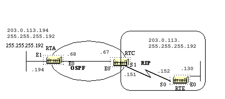
Assume that RTE injects a default-route 0.0.0.0 into RIP. RTC has a gateway of last resort of 203.0.113.152. RTC does not propagate the default to RTA until we configure RTC with a default-information originate command.
RTC#show ip route
 Codes: C - connected, S - static, I - IGRP, R - RIP, M - mobile, B - BGP
        D - EIGRP, EX - EIGRP external, O - OSPF, IA - OSPF inter area
        E1 - OSPF external type 1, E2 - OSPF external type 2, E - EGP
        i - IS-IS, L1 - IS-IS level-1, L2 - IS-IS level-2, * - candidate default

 Gateway of last resort is 203.0.113.152 to network 0.0.0.0

      203.0.113.150 255.255.255.192 is subnetted, 4 subnets
 C       203.0.113.150 is directly connected, Serial1
 C       203.0.113.64 is directly connected, Ethernet0
 R       203.0.113.15128 [120/1] via 203.0.113.152, 00:00:17, Serial1
 O       203.0.113.15192 [110/20] via 203.0.113.68, 2d23, Ethernet0
 R*   0.0.0.0 0.0.0.0 [120/1] via 203.0.113.152, 00:00:17, Serial1
             [120/1] via 203.0.113.68, 00:00:32, Ethernet0
 RTC#

 interface Ethernet0
  ip address 203.0.113.67 255.255.255.192

 interface Serial1
  ip address 203.0.113.151 255.255.255.192

 router ospf 10
  redistribute rip metric 10 subnets
  network 203.0.113.150 0.0.0.255 area 0
  default-information originate metric 10


 router rip
  redistribute ospf 10 metric 2
  passive-interface Ethernet0
  network 203.0.113.150

RTA#show ip route

 Codes: C - connected, S - static, I - IGRP, R - RIP, M - mobile, B - BGP
        D - EIGRP, EX - EIGRP external, O - OSPF, IA - OSPF inter area
        E1 - OSPF external type 1, E2 - OSPF external type 2, E - EGP
        i - IS-IS, L1 - IS-IS level-1, L2 - IS-IS level-2, * - candidate default

 Gateway of last resort is 203.0.113.67 to network 0.0.0.0

      203.0.113.150 255.255.255.192 is subnetted, 4 subnets
 O       203.0.113.150 [110/74] via 203.0.113.67, 2d23, Ethernet0
 C       203.0.113.64 is directly connected, Ethernet0
 O E2    203.0.113.15128 [110/10] via 203.0.113.67, 2d23, Ethernet0
 C       203.0.113.15192 is directly connected, Ethernet1
 O*E2 0.0.0.0 0.0.0.0 [110/10] via 203.0.113.67, 00:00:17, Ethernet0
Note that RTA has learned 0.0.0.0 as an external route with metric 10. The gateway of last resort is set to 203.0.113.67 as expected.
OSPF Design Tips
The OSPF RFC (1583) did not specify any guidelines for the number of routers in an area or number the of neighbors per segment or what is the best way to architect a network.
There are different approaches to OSPF network design. The important thing to remember is that any protocol can fail under pressure.
The idea is not to challenge the protocol but rather to work with it in order to get the best behavior.
Number of Routers per Area
The maximum number of routers per area depends on several factors:
- What kind of area do you have?
- What kind of CPU power do you have in that area?
- What kind of media?
- Does OSPF run in NBMA mode?
- Is your NBMA network meshed?
- Do you have a lot of external LSAs in the network?
- Are other areas well summarized?
For this reason, it is difficult to specify a maximum number of routers per area. Consult your local sales or system engineer for specific network design help.
Number of Neighbors
The number of routers connected to the same LAN is also important. Each LAN has a DR and BDR that build adjacencies with all other routers.
The fewer neighbors that exist on the LAN, the smaller the number of adjacencies a DR or BDR have to build. That depends on how much power your router has.
You could always change the OSPF priority to select your DR. Avoid the same router as DR on more than one segment.
If DR selection is based on the highest RID, then one router could accidently become a DR over all segments it is connected to. This router requires extra effort while other routers are idle.
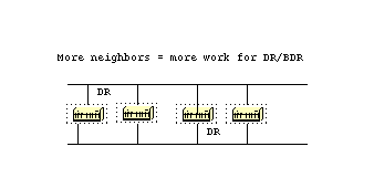
Number of Areas per ABR
ABRs keep a copy of the database for all areas they service. If a router is connected to five areas for example, it has to keep a list of five different databases.
The number of areas per ABR is a number that is dependent on many factors, which includetype of area (normal, stub, NSSA), ABR CPU power, number of routes per area, and number of external routes per area.
For this reason, a specific number of areas per ABR cannot be recommended. It is not preferable to overload an ABR when you can always spread the areas over other routers.
This diagram shows the difference between one ABR which holds five different databases (which includes area 0) and two ABRs which hold three databases each.
These are just guidelines. More areas configured per ABR result in lower performance. In some cases, the lower performance can be tolerated.
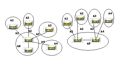
Full Mesh vs. Partial Mesh
The combination of low bandwidth and too many link-states (associated with Non Broadcast Multi-Access (NBMA) clouds such as Frame Relay or X.25) are always a challenge
A partial mesh topology has proven to behave much better than a full mesh. A carefully laid out point-to-point or point-to-multipoint network works much better than multipoint networks that have to deal with DR issues.
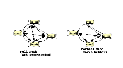
Memory Issues
It is not easy to figure out the memory needed for a particular OSPF configuration. Memory issues usually come up when too many external routes are injected in the OSPF domain.
A backbone area with 40 routers and a default route to the outside world would have less memory issues compared with a backbone area with 4 routers and 33,000 external routes injected into OSPF.
Memory is also conserved through good OSPF design. Summarization at the area border routers and use of stub areas could further minimize the number of routes exchanged.
The total memory used by OSPF is the sum of the memory used in the routing table (show ip route summary) and the memory used in the link-state database.
The numbers are a rule of thumb estimate. Each entry in the routing table consumes between approximately 200 and 280 bytes plus 44 bytes per extra path.
Each LSA consumes a 100 byte overhead plus the size of the actual link state advertisement, possibly another 60 to 100 bytes (for router links, this depends on the number of interfaces on the router).
This must be added to memory used by other processes and by the Cisco IOS® itself. To know the exact number, run show memory with and without OSPF turned on.
The difference in the processor memory used would be the answer (keep a backup copy of the configs).
Normally, a routing table with less than 500K bytes could be accommodated with 2 to 4 MB RAM; Large networks with greater than 500K need 8 to 16 MB, or 32 to 64 MB if full routes are injected from the Internet.
Summary
The OSPF protocol defined in RFC 1583, provides a high functionality open protocol that allows multiple vendor networks to communicate with the TCP/IP protocol family.
Some of the benefits of OSPF are, fast convergence, VLSM, authentication, hierarchical segmentation, route summarization, and aggregation which are needed to handle large and complicated networks.
Appendix A: Link-State Database Synchronization
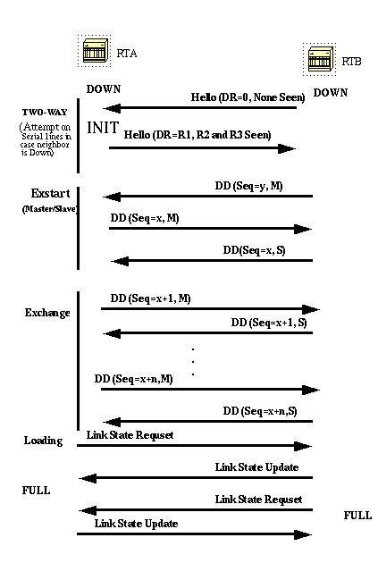
In this diagram, routers on the same segment go through a series of states before they form a successful adjacency. The neighbor and DR election are done via the Hello protocol.
When a router sees itself in its neighbor Hello packet, the state transitions to «2-Way». At that point DR and BDR election is performed on multi-access segments.
A router continues to form an adjacency with a neighbor if either of the two routers is a DR or BDR or they are connected via a point-to-point or virtual link.
In the Exstart state,the two neighbors form a primary/secondary relationship where they agree on a initial sequence number. The sequence number is used to detect old or duplicate Link-State Advertisements (LSA).
In the Exchange state, Database Description Packets (DD) gets exchanged. These are abbreviated link-state advertisements in the form of link-state headers. The header supplies enough information to identify a link.
The primary node sends DD packets which are acknowledged with DD packets from the secondary node. All adjacencies in exchange state or greater are used by the flood procedure.
These adjacencies are fully capable of transmission and reception of all types of OSPF routing protocol packets.
In the Load state, link-state request packets are sent to neighbors, to ask for more recent advertisements that have been discovered but not yet received. Each router builds a list of required LSAs to bring its adjacency up to date.
A Retransmission List is maintained to make sure that every LSA is acknowledged. To specify the number of seconds between link-state advertisement retransmissions for the adjacency you can use:
ip ospf retransmit-interval seconds
Link-state update packets are sent in response to request packets. The link-state update packets are flooded over all adjacencies.
In the Full state, the neighbor routers are fully adjacent. The databases for a common area are an exact match between adjacent routers.
Each LSA has an age field that gets periodically incremented while it is contained in the database or as it gets flooded throughout the area. When an LSA reaches a Maxage it gets flushed from the database if that LSA is not on any neighbors retransmission list.
Link-State Advertisements
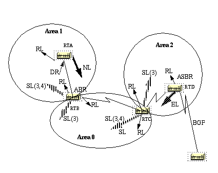
Link-state advertisements are broken into five types. Router Links (RL) are generated by all routers. These links describe the state of the router interfaces inside a particular area.
These links are only flooded inside the router area. Network Links (NL) are generated by a DR of a particular segment; these are an indication of the routers connected to that segment.
Summary Links (SL) are the inter-area links (type 3); these links list the networks inside other areas but still belong to the autonomous system.
Summary links are injected by the ABR from the backbone into other areas and from other areas into the backbone. These links are used for aggregation between areas.
Other types of summary links are the asbr-summary links. These are type 4 links that point to the ASBR. This is to make sure that all routers know the way to exit the autonomous system.
The last type is type 5, External Links (EL), these are injected by the ASBR into the domain.
The previous diagram illustrates the different link types. RTA generates a router link (RL) into area 1, and it also generates a network link (NL) since it happens the be the DR on that particular segment.
RTB is an ABR, and it generates RL into area 1 and area 0. RTB also generates summary links into area 1 and area 0. These links are the list of networks that are interchanged between the two areas.
An ASBR summary link is also injected by RTB into area 1. This is an indication of the existence of RTD, the autonomous system boundary router (ASBR).
Similarly RTC, which is another ABR, generates RL for area 0 and area 2, and a SL (3) into area 2 (since it does not announce any ASBR), and a SL (3,4) into area 0 to announce RTD.
RTD generates a RL for area 2 and generates an EL for external routes learned via BGP. The external routers are flooded all over the domain.
This table is a summary of the link state advertisements.
| LS Type | Advertisement Description |
|---|---|
| 1 | Router Link advertisements. Generated by each router for each area it belongs to. They describe the states of the router link to the area. These are only flooded within a particular area. |
| 2 | Network Link advertisements. Generated by Designated Routers. They describe the set of routers attached to a particular network. Flooded in the area that contains the network. |
| 3 or 4 | Summary Link advertisements. Generated by Area Border routers. They describe inter-area (between areas) routes. Type 3 describes routes to networks, also used to aggregate routes. Type 4 describes routes to ASBR. |
| 5 | AS external link advertisements. Originated by ASBR. They describe routes to destinations external to the AS. Flooded all over except stub areas. |
If you look at the OSPF database in detail, with show ip ospf database detail, there are different keywords such as Link-Data, Link-ID, and Link-state ID. These terms become inconsistent as the value of each depends on the link state type and the link-type.
We review this terminology and provide a detailed example on the OSPF database as seen from the router.
The Link-State ID basically defines the identity of the link-state depending on the LS type.
Router Links are identified by the router ID (RID) of the router that originated the advertisement.
Network Links are identified by the relative IP address of the DR. This makes sense because Network Links are originated by the Designated Router.
Summary Links (type 3) are identified by the IP network numbers of the destinations to which they point.
ASBR Summary Links (Summary Links type 4) are identified by the RID of the ASBR.
External Links are identified by the IP network numbers of the external destinations to which they point. This table summarizes this information:
| LS Type | Link State ID (In the high level view of the database when a router is referenced, this is called Link ID) |
|---|---|
| 1 | The origin Router ID (RID). |
| 2 | The IP interface address of the network Designated Router. |
| 3 | The destination network number. |
| 4 | The router ID of the described AS boundary router. |
| 5 | The external network number. |
The different links available:
Stub network links: This term has nothing to do with stub areas. A stub segment is a segment that has one router only attached to it.
An Ethernet or Token Ring segment that has one attached router is considered a link to a stub network. A loopback interface is also considered a link to stub network with a 255.255.255.255 mask (Host route).
Point-to-point links: These could be physical or logical (subinterfaces) point-to-point serial link connections. These links could be numbered (an IP address is configured on the link) or unnumbered.
Transit links: These are interfaces connected to networks that have more than one router attached, hence the name transit.
Virtual links: These are logical links that connect areas that do not have physical connections to the backbone. Virtual links are treated as numbered point-to-point links.
The link-ID is an identification of the link itself. This is different for each link type.
A transit link is identified by the IP address of the DR on that link.
A numbered point-to-point link is identified by the RID of the neighbor router on the point-to-point link.
Virtual links are identical to point-to-point links.
Stub network links are identified by the IP address of the interface to the stub network. This table summarizes this information:
| Link Type | Link ID (This applies to individual Links) |
|---|---|
| Point-to-Point | Neighbor Router ID |
| Link to transit network | Interface address of DR |
| Link to stub network (In case of loopback mask is 255.255.255.255) | Network/subnet number |
| Virtual Link | Neighbor Router ID |
The Link Data is the IP address of the link, except for stub network where the link data is the network mask.
| Link Type | Link Data |
|---|---|
| Stub network | Network Mask |
| Other networks (applies to router links only) | Router — associated IP interface address |
Finally, an Advertising Router is the RID of the router that has sent the LSA.
OSPF Database Example
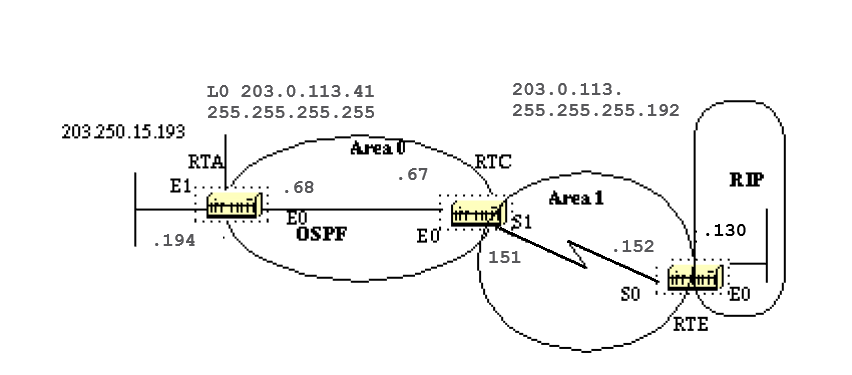
Given this network diagram, the configurations, and the IP route tables, here are different ways to understand the OSPF database.
RTA#
 interface Loopback0
  ip address 203.0.113.41 255.255.255.255

 interface Ethernet0
  ip address 203.0.113.68 255.255.255.192

 interface Ethernet1
  ip address 203.0.113.15193 255.255.255.192

 router ospf 10
  network 203.0.113.100 0.0.255.255 area 0

 RTA#show ip route
 Codes: C - connected, S - static, I - IGRP, R - RIP, M - mobile, B - BGP
        D - EIGRP, EX - EIGRP external, O - OSPF, IA - OSPF inter area
        E1 - OSPF external type 1, E2 - OSPF external type 2, E - EGP
        i - IS-IS, L1 - IS-IS level-1, L2 - IS-IS level-2, * - candidate default

 Gateway of last resort is 203.0.113.67 to network 0.0.0.0

      203.0.113.128 255.255.255.192 is subnetted, 1 subnets
 O E2    203.0.113.1288 [110/10] via 203.0.113.67, 00:00:50, Ethernet0
      203.0.113.30 255.255.255.255 is subnetted, 1 subnets
 C       203.0.113.41 is directly connected, Loopback0
      203.0.113.150 255.255.255.192 is subnetted, 3 subnets
 O IA    203.0.113.150 [110/74] via 203.0.113.67, 00:00:50, Ethernet0
 C       203.0.113.64 is directly connected, Ethernet0
 C       203.0.113.15192 is directly connected, Ethernet1
 O*E2 0.0.0.0 0.0.0.0 [110/10] via 203.0.113.67, 00:00:50, Ethernet0

 RTE#
 ip subnet-zero

 interface Ethernet0
  ip address 203.0.113.16 255.255.255.192

 interface Serial0
  ip address 203.0.113.152 255.255.255.192

 router ospf 10
  redistribute rip metric 10 subnets
  network 203.0.113.150 0.0.0.63 area 1
  default-information originate metric 10

 router rip
  network 203.0.113.128

 ip route 0.0.0.0 0.0.0.0 Ethernet0

RTE#show ip route
 Codes: C - connected, S - static, I - IGRP, R - RIP, M - mobile, B - BGP
        D - EIGRP, EX - EIGRP external, O - OSPF, IA - OSPF inter area
        E1 - OSPF external type 1, E2 - OSPF external type 2, E - EGP
        i - IS-IS, L1 - IS-IS level-1, L2 - IS-IS level-2, * - candidate default

 Gateway of last resort is 0.0.0.0 to network 0.0.0.0

      203.0.113.128 255.255.255.192 is subnetted, 1 subnets
 C       203.0.113.1288 is directly connected, Ethernet0
      203.0.113.30 is variably subnetted, 2 subnets, 2 masks
 O IA    203.0.113.41 255.255.255.255
            [110/75] via 203.0.113.151, 00:16:31, Serial0
      203.0.113.150 255.255.255.192 is subnetted, 3 subnets
 C       203.0.113.150 is directly connected, Serial0
 O IA    203.0.113.64 [110/74] via 203.0.113.151, 00:16:31, Serial0
 O IA    203.0.113.15192 [110/84] via 203.0.113.151, 00:16:31, Serial0
 S*   0.0.0.0 0.0.0.0 is directly connected, Ethernet0

 RTC#
 ip subnet-zero

 interface Ethernet0
  ip address 203.0.113.67 255.255.255.192

 interface Serial1
  ip address 203.0.113.151 255.255.255.192

 router ospf 10
  network 203.0.113.64 0.0.0.63 area 0
  network 203.0.113.150 0.0.0.63 area 1

RTF#show ip route
 Codes: C - connected, S - static, I - IGRP, R - RIP, M - mobile, B - BGP
        D - EIGRP, EX - EIGRP external, O - OSPF, IA - OSPF inter area
        E1 - OSPF external type 1, E2 - OSPF external type 2, E - EGP
        i - IS-IS, L1 - IS-IS level-1, L2 - IS-IS level-2, * - candidate default

 Gateway of last resort is 203.0.113.152 to network 0.0.0.0

      203.0.113.128 255.255.255.192 is subnetted, 1 subnets
 O E2    203.0.113.1288 [110/10] via 203.0.113.152, 04:49:05, Serial1
      203.0.113.30 255.255.255.255 is subnetted, 1 subnets
 O       203.0.113.41 [110/11] via 203.0.113.68, 04:49:06, Ethernet0
      203.0.113.150 255.255.255.192 is subnetted, 3 subnets
 C       203.0.113.150 is directly connected, Serial1
 C       203.0.113.64 is directly connected, Ethernet0
 O       203.0.113.15192 [110/20] via 203.0.113.68, 04:49:06, Ethernet0
 O*E2 0.0.0.0 0.0.0.0 [110/10] via 203.0.113.152, 04:49:06, Serial1
General View of the Database
RTC#show ip ospf database

       OSPF Router with ID (203.0.113.67) (Process ID 10)

                Router Link States (Area 1)

Link ID         ADV Router      Age    Seq#       Checksum Link count
203.0.113.67   203.0.113.67   48     0x80000008 0xB112   2
203.0.113.16  203.0.113.16  212    0x80000006 0x3F44   2

                Summary Net Link States (Area 1)

Link ID         ADV Router      Age    Seq#       Checksum
203.0.113.41   203.0.113.67   602    0x80000002 0x90AA
203.0.113.64   203.0.113.67   620    0x800000E9 0x3E3C
203.0.113.15192  203.0.113.67   638    0x800000E5 0xA54E

                Router Link States (Area 0)

Link ID         ADV Router      Age    Seq#       Checksum Link count
203.0.113.41   203.0.113.41   179    0x80000029 0x9ADA   3
203.0.113.67   203.0.113.67   675    0x800001E2 0xDD23   1

                Net Link States (Area 0)

Link ID         ADV Router      Age    Seq#       Checksum
203.0.113.68   203.0.113.41   334    0x80000001 0xB6B5

                Summary Net Link States (Area 0)

Link ID         ADV Router      Age    Seq#       Checksum
203.0.113.150    203.0.113.67   792    0x80000002 0xAEBD

                Summary ASB Link States (Area 0)

Link ID         ADV Router      Age    Seq#       Checksum
203.0.113.16  203.0.113.67   579    0x80000001 0xF9AF

                AS External Link States

Link ID         ADV Router      Age    Seq#       Checksum Tag
0.0.0.0         203.0.113.16  1787   0x80000001 0x98CE   10
203.0.113.1288  203.0.113.16  5      0x80000002 0x93C4   0
This is a general look at the whole OSPF database. The database is listed in accord with the areas. In this case, we look at the RTC database which is an ABR. Both area 1 and area 0’s databases are listed.
Area 1 is composed of router links and summary links. No network links exist because no DR exists on any of the segments in area 1. No Summary ASBR links exist in area 1 because the only ASBR happens to be in area 0.
External links do not belong to any particular area as they are flooded all over. Note that all the links are the cumulative links collected from all routers in an area.
Concentrate on the database in area 0. The Link-ID indicated here is actually the Link-State ID. This is a representation of the whole router, not a particular link. This seems ambiguous.
Remember that this high level Link-ID (actually Link-State ID) represents the whole router and not just a link.
Router Links
Router Link States (Area 0)

 Link ID         ADV Router      Age    Seq#       Checksum Link count
 203.0.113.41   203.0.113.41   179    0x80000029 0x9ADA   3
 203.0.113.67   203.0.113.67   675    0x800001E2 0xDD23   1
Start with the router links. There are two entries listed for 203.0.113.41 and 203.0.113.67, these are the RIDs of the two routers in area 0. The number of links in area 0 for each router is also indicated. RTA has three links to area 0 and RTC has one link. A detailed view of the RTC router links:
RTC#show ip ospf database router 203.0.113.67

     OSPF Router with ID (203.0.113.67) (Process ID 10)

                Router Link States (Area 1)

  LS age: 1169
  Options: (No TOS-capability)
  LS Type: Router Links
  Link State ID: 203.0.113.67
  Advertising Router: 203.0.113.67
  LS Seq Number: 80000008
  Checksum: 0xB112
  Length: 48
  Area Border Router
   Number of Links: 2

    Link connected to: another Router (point-to-point)
     (Link ID) Neighbor Router ID: 203.0.113.16
     (Link Data) Router Interface address: 203.0.113.151
      Number of TOS metrics: 0
       TOS 0 Metrics: 64

    Link connected to: a Stub Network
     (Link ID) Network/subnet number: 203.0.113.150
     (Link Data) Network Mask: 255.255.255.192
      Number of TOS metrics: 0
       TOS 0 Metrics: 64
One thing to note here is that OSPF generates an extra stub link for each point-to-point interface. Do not get confused if you see the link count larger than the number of physical interfaces.
Router Link States (Area 0)

  LS age: 1227
  Options: (No TOS-capability)
  LS Type: Router Links
  Link State ID: 203.0.113.67
  Advertising Router: 203.0.113.67
  LS Seq Number: 80000003
  Checksum: 0xA041
  Length: 36
  Area Border Router
   Number of Links: 1

    Link connected to: a Transit Network
     (Link ID) Designated Router address: 203.0.113.68
     (Link Data) Router Interface address: 203.0.113.67
      Number of TOS metrics: 0
       TOS 0 Metrics: 10
Note that the Link ID is equal to the IP address (not the RID) of the attached DR; in this case it is 203.0.113.68. The Link Data is the RTC IP address.
Network Links
Net Link States (Area 0)

Link ID         ADV Router      Age    Seq#       Checksum
203.0.113.68   203.0.113.41   334    0x80000001 0xB6B5
One network link is listed, indicated by the interface IP address (not the RID) of the DR, in this case 203.0.113.68. A detailed view of this entry:
RTC#show ip ospf database network

       OSPF Router with ID (203.0.113.67) (Process ID 10)

                Net Link States (Area 0)

  Routing Bit Set on this LSA
  LS age: 1549
  Options: (No TOS-capability)
  LS Type: Network Links
  Link State ID: 203.0.113.68 (address of Designated Router)
  Advertising Router: 203.0.113.41
  LS Seq Number: 80000002
  Checksum: 0xB4B6
  Length: 32
  Network Mask: 255.255.255.192

        Attached Router: 203.0.113.41
        Attached Router: 203.0.113.67
Note that the network link lists the RIDs of the routers attached to the transit network; in this case the RIDs of RTA and RTC are listed.
Summary Links
Summary Net Link States (Area 0)

Link ID         ADV Router      Age    Seq#       Checksum
203.0.113.150    203.0.113.67   792    0x80000002 0xAEBD
Area 0 has one summary link represented by the IP network address of the
link 203.0.113.150. This link was injected by the ABR RTC from area 1 into
area 0. A detailed view of this summary link, summary links for
area 1 are not listed here:

RTC#show ip ospf database summary (area 1 is not listed)

              Summary Net Link States (Area 0)

  LS age: 615
  Options: (No TOS-capability)
  LS Type: Summary Links(Network)
  Link State ID: 203.0.113.150 (summary Network Number)
  Advertising Router: 203.0.113.67
  LS Seq Number: 80000003
  Checksum: 0xACBE
  Length: 28
  Network Mask: 255.255.255.192 TOS: 0  Metric: 64
Summary ASBR Links
Summary ASB Link States (Area 0)

Link ID         ADV Router      Age    Seq#       Checksum
203.0.113.16  203.0.113.67   579    0x80000001 0xF9AF
This is an indication of who the ASBR is. In this case the ASBR is RTE represented by its RID 203.0.113.16. The advertising router for this entry into area 0 is RTC with RID 203.0.113.67. A detailed view of the summary ASBR entry:
RTC#show ip ospf database asbr-summary

        OSPF Router with ID (203.0.113.67) (Process ID 10)

                 Summary ASB Link States (Area 0)

   LS age: 802
   Options: (No TOS-capability)
   LS Type: Summary Links(AS Boundary Router)
   Link State ID: 203.0.113.16 (AS Boundary Router address)
   Advertising Router: 203.0.113.67
   LS Seq Number: 80000003
   Checksum: 0xF5B1
   Length: 28
   Network Mask: 0.0.0.0 TOS: 0  Metric: 64
External Links
AS External Link States

Link ID         ADV Router      Age    Seq#       Checksum Tag
0.0.0.0         203.0.113.16  1787   0x80000001 0x98CE   10
203.0.113.1288  203.0.113.16  5      0x80000002 0x93C4   0
We have two external Links, the first one is the 0.0.0.0 injected into OSPF via the default-information originate command.
The other entry is network 203.0.113.128 8 which is injected into OSPF by redistribution.
The router advertising these networks is 203.0.113.16, the RID of RTE.
This is the detailed view of the external routes:
RTC#show ip ospf database external

        OSPF Router with ID (203.0.113.67) (Process ID 10)

                 AS External Link States

   Routing Bit Set on this LSA
   LS age: 208
   Options: (No TOS-capability)
   LS Type: AS External Link
   Link State ID: 0.0.0.0 (External Network Number )
   Advertising Router: 203.0.113.16
   LS Seq Number: 80000002
   Checksum: 0x96CF
   Length: 36
   Network Mask: 0.0.0.0
         Metric Type: 2 (Larger than any link state path)
         TOS: 0
         Metric: 10
         Forward Address: 0.0.0.0
         External Route Tag: 10

  Routing Bit Set on this LSA
   LS age: 226
   Options: (No TOS-capability)
   LS Type: AS External Link
   Link State ID: 203.0.113.1288 (External Network Number)
   Advertising Router: 203.0.113.16
   LS Seq Number: 80000002
   Checksum: 0x93C4
   Length: 36
   Network Mask: 255.255.255.192
         Metric Type: 2 (Larger than any link state path)
         TOS: 0
         Metric: 10
         Forward Address: 0.0.0.0
         External Route Tag: 0
Note the forward address. Whenever this address is 0.0.0.0 it indicates that the external routes are reachable via the advertising router, in this case 203. 250.16.130.
This is why the identity of the ASBR is injected by ABRs into other areas which use ASBR summary links.
This forward address is not always 0.0.0.0. In some cases, it could be the IP address of another router on the same segment. This diagram illustrates this situation:
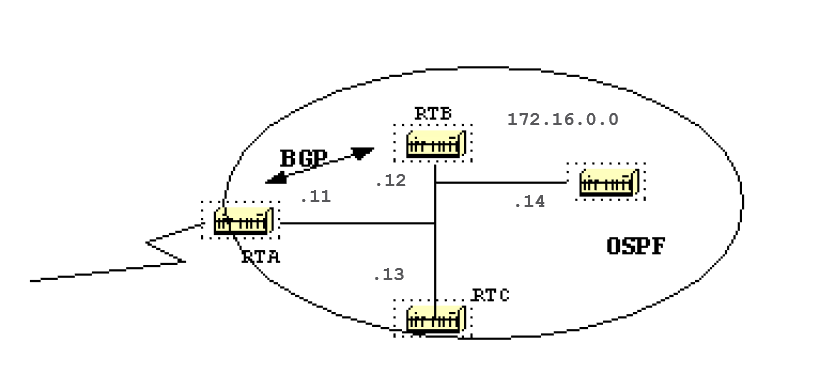
In this situation RTB, runs BGP with RTA, and OSPF with the rest of the domain. RTA does not run OSPF. RTB redistributes BGP routes into OSPF.
In accord with OSPF, RTB is an ASBR advertising external routes. The forwarding address in this case is set to 172.16.0.11 and not to the advertising router (0.0.0.0) RT B.
There is no need to make the extra hop. Routers inside the OSPF domain must reach the forwarding address via OSPF in order for the external routes to be put in the IP routing table.
If the forwarding address is reached via some other protocol or no t accessible, the external entries would be in the database but not in the IP routing table.
Another situation would arise if both RTB and RTC are ASBRs (RTC runs BGP with RTA). In this situation, in order to eliminate the duplication of the effort, one of the two routers do not advertise (flushes) the external routes. The router with the higher RID prevails.
The Full Database
This is a list of the whole database as an exercise. You are now able to review and explain each entry:
RTC#show ip ospf database router

         OSPF Router with ID (203.0.113.67) (Process ID 10)

                 Router Link States (Area 1)

   LS age: 926
   Options: (No TOS-capability)
   LS Type: Router Links
   Link State ID: 203.0.113.67
   Advertising Router: 203.0.113.67
   LS Seq Number: 80000035
   Checksum: 0x573F
   Length: 48
   Area Border Router
    Number of Links: 2
     Link connected to: another Router (point-to-point)
      (Link ID) Neighbor Router ID: 203.0.113.16
      (Link Data) Router Interface address: 203.0.113.151
       Number of TOS metrics: 0
        TOS 0 Metrics: 64

     Link connected to: a Stub Network
      (Link ID) Network/subnet number: 203.0.113.150
      (Link Data) Network Mask: 255.255.255.192
       Number of TOS metrics: 0
        TOS 0 Metrics: 64

   Routing Bit Set on this LSA
   LS age: 958
   Options: (No TOS-capability)
   LS Type: Router Links
   Link State ID: 203.0.113.16
   Advertising Router: 203.0.113.16
   LS Seq Number: 80000038
   Checksum: 0xDA76
   Length: 48
   AS Boundary Router
    Number of Links: 2

     Link connected to: another Router (point-to-point)
      (Link ID) Neighbor Router ID: 203.0.113.67
      (Link Data) Router Interface address: 203.0.113.152
       Number of TOS metrics: 0
        TOS 0 Metrics: 64

     Link connected to: a Stub Network
      (Link ID) Network/subnet number: 203.0.113.150
      (Link Data) Network Mask: 255.255.255.192
       Number of TOS metrics: 0
        TOS 0 Metrics: 64

                 Router Link States (Area 0)

   Routing Bit Set on this LSA
   LS age: 1107
   Options: (No TOS-capability)
   LS Type: Router Links
   Link State ID: 203.0.113.41
   Advertising Router: 203.0.113.41
   LS Seq Number: 8000002A
   Checksum: 0xC0B0
   Length: 60
   AS Boundary Router
    Number of Links: 3

     Link connected to: a Stub Network
      (Link ID) Network/subnet number: 203.0.113.41
      (Link Data) Network Mask: 255.255.255.255
       Number of TOS metrics: 0
        TOS 0 Metrics: 1

     Link connected to: a Stub Network
      (Link ID) Network/subnet number: 203.0.113.15192
      (Link Data) Network Mask: 255.255.255.192
       Number of TOS metrics: 0
        TOS 0 Metrics: 10

     Link connected to: a Transit Network
      (Link ID) Designated Router address: 203.0.113.68
      (Link Data) Router Interface address: 203.0.113.68
       Number of TOS metrics: 0
        TOS 0 Metrics: 10

   LS age: 1575
   Options: (No TOS-capability)
   LS Type: Router Links
   Link State ID: 203.0.113.67
   Advertising Router: 203.0.113.67
   LS Seq Number: 80000028
   Checksum: 0x5666
   Length: 36
   Area Border Router
    Number of Links: 1

     Link connected to: a Transit Network
      (Link ID) Designated Router address: 203.0.113.68
      (Link Data) Router Interface address: 203.0.113.67
       Number of TOS metrics: 0
        TOS 0 Metrics: 10

 RTC#show ip ospf database network

        OSPF Router with ID (203.0.113.67) (Process ID 10)

                 Net Link States (Area 0)

   Routing Bit Set on this LSA
   LS age: 1725
   Options: (No TOS-capability)
   LS Type: Network Links
   Link State ID: 203.0.113.68 (address of Designated Router)
   Advertising Router: 203.0.113.41
   LS Seq Number: 80000026
   Checksum: 0x6CDA
   Length: 32
   Network Mask: 255.255.255.192
         Attached Router: 203.0.113.41
         Attached Router: 203.0.113.67

 RTC#show ip ospf database summary

        OSPF Router with ID (203.0.113.67) (Process ID 10)

                 Summary Net Link States (Area 1)

   LS age: 8
   Options: (No TOS-capability)
   LS Type: Summary Links(Network)
   Link State ID: 203.0.113.41 (summary Network Number)
   Advertising Router: 203.0.113.67
   LS Seq Number: 80000029
   Checksum: 0x42D1
   Length: 28
   Network Mask: 255.255.255.255 TOS: 0  Metric: 11

   LS age: 26
   Options: (No TOS-capability)
   LS Type: Summary Links(Network)
   Link State ID: 203.0.113.64 (summary Network Number)
   Advertising Router: 203.0.113.67
   LS Seq Number: 80000030
   Checksum: 0xB182
   Length: 28
   Network Mask: 255.255.255.192 TOS: 0  Metric: 10

   LS age: 47
   Options: (No TOS-capability)
   LS Type: Summary Links(Network)
   Link State ID: 203.0.113.15192 (summary Network Number)
   Advertising Router: 203.0.113.67
   LS Seq Number: 80000029
   Checksum: 0x1F91
   Length: 28
   Network Mask: 255.255.255.192 TOS: 0  Metric: 20

                 Summary Net Link States (Area 0)

   LS age: 66
   Options: (No TOS-capability)
   LS Type: Summary Links(Network)
   Link State ID: 203.0.113.150 (summary Network Number)
   Advertising Router: 203.0.113.67
   LS Seq Number: 80000025
   Checksum: 0x68E0
   Length: 28
   Network Mask: 255.255.255.192 TOS: 0  Metric: 64

 RTC#show ip ospf asbr-summary

        OSPF Router with ID (203.0.113.67) (Process ID 10)

                 Summary ASB Link States (Area 0)

   LS age: 576
   Options: (No TOS-capability)
   LS Type: Summary Links(AS Boundary Router)
   Link State ID: 203.0.113.16 (AS Boundary Router address)
   Advertising Router: 203.0.113.67
   LS Seq Number: 80000024
   Checksum: 0xB3D2
   Length: 28
   Network Mask: 0.0.0.0 TOS: 0  Metric: 64


 RTC#show ip ospf database external

       OSPF Router with ID (203.0.113.67) (Process ID 10)

                 AS External Link States

   Routing Bit Set on this LSA
   LS age: 305
   Options: (No TOS-capability)
   LS Type: AS External Link
   Link State ID: 0.0.0.0 (External Network Number)
   Advertising Router: 203.0.113.16
   LS Seq Number: 80000001
   Checksum: 0x98CE
   Length: 36
   Network Mask: 0.0.0.0
         Metric Type: 2 (Larger than any link state path)
         TOS: 0
         Metric: 10
         Forward Address: 0.0.0.0
         External Route Tag: 10

   Routing Bit Set on this LSA
   LS age: 653
   Options: (No TOS-capability)
   LS Type: AS External Link
   Link State ID: 203.0.113.1288 (External Network Number)
   Advertising Router: 203.0.113.16
   LS Seq Number: 80000024
   Checksum: 0x4FE6
   Length: 36
   Network Mask: 255.255.255.192
         Metric Type: 2 (Larger than any link state path)
         TOS: 0
         Metric: 10
         Forward Address: 0.0.0.0
         External Route Tag: 0
Appendix B: OSPF and IP Multicast Address
OSPF used IP multicast to exchange Hello packets and Link State Updates. An IP multicast address is implemented with class D addresses. A class D address ranges from 224.0.0.0 to 239.255.255.255.
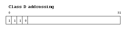
Some special IP multicast addresses are reserved for OSPF:
- 224.0.0.5: All OSPF routers must be able to transmit and listen to this address.
- 224.0.0.6: All DR and BDR routers must be able to transmit and listen to this address.
The mapping between IP multicast addresses and MAC addresses has the rule:
For multiaccess networks that support multicast, the low order 23 bits of the IP address are used as the low order bits of the MAC multicast address 01-005E-00-00- 00. For example:
- 224.0.0.5 would be mapped to 01-00-5E-00-00-05
- 224.0.0.6 would be mapped to 01-00-5E-00-00-06
OSPF uses broadcast on Token Ring networks.
Appendix C: Variable Length Subnet Masks (VLSM)
This is a binary/decimal conversion chart:
| 0000 | 0001 | 0010 | 0011 | 0100 | 0101 | 0110 | 0111 | ||||||||
|---|---|---|---|---|---|---|---|---|---|---|---|---|---|---|---|
| 0 | 0000 | 16 | 0000 | 32 | 0000 | 48 | 0000 | 64 | 0000 | 80 | 0000 | 96 | 0000 | 112 | 0000 |
| 1 | 0001 | 17 | 0001 | 33 | 0001 | 49 | 0001 | 65 | 0001 | 81 | 0001 | 97 | 0001 | 113 | 0001 |
| 2 | 0010 | 18 | 0010 | 34 | 0010 | 50 | 0010 | 66 | 0010 | 82 | 0010 | 98 | 0010 | 114 | 0010 |
| 3 | 0011 | 19 | 0011 | 35 | 0011 | 51 | 0011 | 67 | 0011 | 83 | 0011 | 99 | 0011 | 115 | 0011 |
| 4 | 0100 | 20 | 0100 | 36 | 0100 | 52 | 0100 | 68 | 0100 | 84 | 0100 | 100 | 0100 | 116 | 0100 |
| 5 | 0101 | 21 | 0101 | 37 | 0101 | 53 | 0101 | 69 | 0101 | 85 | 0101 | 101 | 0101 | 117 | 0101 |
| 6 | 0110 | 22 | 0110 | 38 | 0110 | 54 | 0110 | 70 | 0110 | 86 | 0110 | 102 | 0110 | 118 | 0110 |
| 7 | 0111 | 23 | 0111 | 39 | 0111 | 55 | 0111 | 71 | 0111 | 87 | 0111 | 103 | 0111 | 119 | 0111 |
| 8 | 1000 | 24 | 1000 | 40 | 1000 | 56 | 1000 | 72 | 1000 | 88 | 1000 | 104 | 1000 | 120 | 1000 |
| 9 | 1001 | 25 | 1001 | 41 | 1001 | 57 | 1001 | 73 | 1001 | 89 | 1001 | 105 | 1001 | 121 | 1001 |
| 10 | 1010 | 26 | 1010 | 42 | 1010 | 58 | 1010 | 74 | 1010 | 90 | 1010 | 106 | 1010 | 122 | 1010 |
| 11 | 1011 | 27 | 1011 | 43 | 1011 | 59 | 1011 | 75 | 1011 | 91 | 1011 | 107 | 1011 | 123 | 1011 |
| 12 | 1100 | 28 | 1100 | 44 | 1100 | 60 | 1100 | 76 | 1100 | 92 | 1100 | 108 | 1100 | 124 | 1100 |
| 13 | 1101 | 29 | 1101 | 45 | 1101 | 61 | 1101 | 77 | 1101 | 93 | 1101 | 109 | 1101 | 125 | 1101 |
| 14 | 1110 | 30 | 1110 | 46 | 1110 | 62 | 1110 | 78 | 1110 | 94 | 1110 | 110 | 1110 | 126 | 1110 |
| 15 | 1111 | 31 | 1111 | 47 | 1111 | 63 | 1111 | 79 | 1111 | 95 | 1111 | 111 | 1111 | 127 | 1111 |
| 1000 | 1001 | 1010 | 1011 | 1100 | 1101 | 1110 | 1111 | ||||||||
| 128 | 0000 | 144 | 0000 | 160 | 0000 | 176 | 0000 | 192 | 0000 | 208 | 0000 | 224 | 0000 | 240 | 0000 |
| 129 | 0001 | 145 | 0001 | 161 | 0001 | 177 | 0001 | 193 | 0001 | 209 | 0001 | 225 | 0001 | 241 | 0001 |
| 130 | 0010 | 146 | 0010 | 162 | 0010 | 178 | 0010 | 194 | 0010 | 210 | 0010 | 226 | 0010 | 242 | 0010 |
| 131 | 0011 | 147 | 0011 | 163 | 0011 | 179 | 0011 | 195 | 0011 | 211 | 0011 | 227 | 0011 | 243 | 0011 |
| 132 | 0100 | 148 | 0100 | 164 | 0100 | 180 | 0100 | 196 | 0100 | 212 | 0100 | 228 | 0100 | 244 | 0100 |
| 133 | 0101 | 149 | 0101 | 165 | 0101 | 181 | 0101 | 197 | 0101 | 213 | 0101 | 229 | 0101 | 245 | 0101 |
| 134 | 0110 | 150 | 0110 | 166 | 0110 | 182 | 0110 | 198 | 0110 | 214 | 0110 | 230 | 0110 | 246 | 0110 |
| 135 | 0111 | 151 | 0111 | 167 | 0111 | 183 | 0111 | 199 | 0111 | 215 | 0111 | 231 | 0111 | 247 | 0111 |
| 136 | 1000 | 152 | 1000 | 168 | 1000 | 184 | 1000 | 200 | 1000 | 216 | 1000 | 232 | 1000 | 248 | 1000 |
| 137 | 1001 | 153 | 1001 | 169 | 1001 | 185 | 1001 | 201 | 1001 | 217 | 1001 | 233 | 1001 | 249 | 1001 |
| 138 | 1010 | 154 | 1010 | 170 | 1010 | 186 | 1010 | 202 | 1010 | 218 | 1010 | 234 | 1010 | 250 | 1010 |
| 139 | 1011 | 155 | 1011 | 171 | 1011 | 187 | 1011 | 203 | 1011 | 219 | 1011 | 235 | 1011 | 251 | 1011 |
| 140 | 1100 | 156 | 1100 | 172 | 1100 | 188 | 1100 | 204 | 1100 | 220 | 1100 | 236 | 1100 | 252 | 1100 |
| 141 | 1101 | 157 | 1101 | 173 | 1101 | 189 | 1101 | 205 | 1101 | 221 | 1101 | 237 | 1101 | 253 | 1101 |
| 142 | 1110 | 158 | 1110 | 174 | 1110 | 190 | 1110 | 206 | 1110 | 222 | 1110 | 238 | 1110 | 254 | 1110 |
| 143 | 1111 | 159 | 1111 | 175 | 1111 | 191 | 1111 | 207 | 1111 | 223 | 1111 | 239 | 1111 | 255 | 1111 |
The idea behind variable length subnet masks is to offer more flexibility to divide a major net into multiple subnets and remain able to maintain an adequate number of hosts in each subnet.
Without VLSM, one subnet mask only can be applied to a major network. This restricts the number of hosts given the number of subnets required.
If you pick the mask such that you have enough subnets, you are not able to allocate enough hosts in each subnet. The same is true for the hosts; a mask that allows enough hosts does not provide enough subnet space.
For example, suppose you were assigned a class C network 192.168.0.0 and you need to divide that network into three subnets with 100 hosts in one subnet and 50 hosts for the remainder of the subnets.
Ignore the two end limits 0 and 255, and you have theoretically available to you 256 addresses (192.168.0.0 — 192.168.0.255). This cannot be done without VLSM.
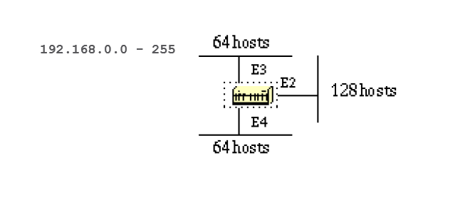
There are a handful of subnet masks that can be used; note that a mask must have a contiguous number of ones that start from the left and the rest of the bits are all 0s.
-252 (1111 1100) The address space is divided into 64.
 -248 (1111 1000) The address space is divided into 32.
 -240 (1111 0000) The address space is divided into 16.
 -224 (1110 0000) The address space is divided into 8.
 -192 (1100 0000) The address space is divided into 4.
 -128 (1000 0000) The address space is divided into 2.
Without VLSM you have the choice to use mask 255.255.255.128 and divide the addresses into 2 subnets with 128 hosts each or use 255.255.255.192 and divide the space into 4 subnets with 64 hosts each.
This does not meet the requirement. If you use multiple masks, you can use mask 128 and further subnet the second chunk of addresses with mask 192.
This table shows how you have divided the address space:
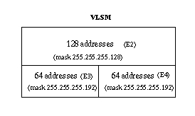
Use caution in the allocation of IP addresses to each mask. Once you assign an IP address to the router or to a host, you have used up the whole subnet for that segment.
For example, if you assign 192.168.0.10 255.255.255.128 to E2, the whole range of addresses between 192.168.0.0 and 192.168.0.127 is consumed by E2.
In the same way if you assign 192.168.0.160 255.255.255.128 to E2, the whole range of addresses between 192.168.0.128 and 192.168.0.255 is consumed by the E2 segment.
This is an illustration of how the router interprets these addresses. Remember that any time you use a mask different than the natural mask, for instance to create a subnet, the router complains if the combination IP address and mask result in a subnet zero.
Use the ip subnet-zero command on the router in order to resolve this issue.
RTA#
 ip subnet-zero
 interface Ethernet2
  ip address 192.168.0.10 255.255.255.128
 interface Ethernet3
  ip address 192.168.0.160 255.255.255.192
 interface Ethernet4
  ip address 192.168.0.226 255.255.255.192

 RTA#show ip route connected
      192.168.0.0  is variably subnetted, 3 subnets, 2 masks
 C       192.168.0.0  255.255.255.128 is directly connected, Ethernet2
 C       192.168.0.128 255.255.255.192 is directly connected, Ethernet3
 C       192.168.0.192 255.255.255.192 is directly connected, Ethernet4
Related Information
- Cisco IOS® IP Routing: OSPF Command Reference
- OSPF and MTU
- OSPF neighbors are stuck in exstart and exchange state due to MTU mismatch
- OSPF Support Page
- OSPF: Frequently Asked Questions
- Technical Support & Documentation — Cisco Systems
| Communication protocol | |
| Purpose | Routing protocol |
|---|---|
| Introduction | 1989; 34 years ago |
| RFC(s) | 1131, 1247, 1583, 2178, 2328, 3101, 5709, 6549, 6845… |
| Communication protocol | |
| Introduction | 1999; 24 years ago |
|---|---|
| RFC(s) | 2740, 5340, 6845, 6860, 7503, 8362… |
Open Shortest Path First (OSPF) is a routing protocol for Internet Protocol (IP) networks. It uses a link state routing (LSR) algorithm and falls into the group of interior gateway protocols (IGPs), operating within a single autonomous system (AS).
OSPF gathers link state information from available routers and constructs a topology map of the network. The topology is presented as a routing table to the internet layer for routing packets by their destination IP address. OSPF supports Internet Protocol version 4 (IPv4) and Internet Protocol version 6 (IPv6) networks and is widely used in large enterprise networks. IS-IS, another LSR-based protocol, is more common in large service provider networks.
Originally designed in the 1980s, OSPF version 2 is defined in RFC 2328 (1998).[1] The updates for IPv6 are specified as OSPF version 3 in RFC 5340 (2008).[2] OSPF supports the Classless Inter-Domain Routing (CIDR) addressing model.
Concepts[edit]
OSPF is an interior gateway protocol (IGP) for routing Internet Protocol (IP) packets within a single routing domain, such as an autonomous system. It gathers link state information from available routers and constructs a topology map of the network. The topology is presented as a routing table to the internet layer which routes packets based solely on their destination IP address.
OSPF detects changes in the topology, such as link failures, and converges on a new loop-free routing structure within seconds.[3] It computes the shortest-path tree for each route using a method based on Dijkstra’s algorithm. The OSPF routing policies for constructing a route table are governed by link metrics associated with each routing interface. Cost factors may be the distance of a router (round-trip time), data throughput of a link, or link availability and reliability, expressed as simple unitless numbers. This provides a dynamic process of traffic load balancing between routes of equal cost.
OSPF divides the network into routing areas to simplify administration and optimize traffic and resource utilization. Areas are identified by 32-bit numbers, expressed either simply in decimal, or often in the same octet-based dot-decimal notation used for IPv4 addresses. By convention, area 0 (zero), or 0.0.0.0, represents the core or backbone area of an OSPF network. While the identifications of other areas may be chosen at will, administrators often select the IP address of a main router in an area as the area identifier. Each additional area must have a connection to the OSPF backbone area. Such connections are maintained by an interconnecting router, known as an area border router (ABR). An ABR maintains separate link-state databases for each area it serves and maintains summarized routes for all areas in the network.
OSPF runs over IPv4 and IPv6, but does not use a transport protocol such as UDP or TCP. It encapsulates its data directly in IP packets with protocol number 89. This is in contrast to other routing protocols, such as the Routing Information Protocol (RIP) and the Border Gateway Protocol (BGP). OSPF implements its own transport error detection and correction functions. OSPF also uses multicast addressing for distributing route information within a broadcast domain. It reserves the multicast addresses 224.0.0.5 (IPv4) and FF02::5 (IPv6) for all SPF/link state routers (AllSPFRouters) and 224.0.0.6 (IPv4) and FF02::6 (IPv6) for all Designated Routers (AllDRouters).[4][5] For non-broadcast networks, special provisions for configuration facilitate neighbor discovery.[1] OSPF multicast IP packets never traverse IP routers, they never travel more than one hop. The protocol may therefore be considered a link layer protocol, but is often also attributed to the application layer in the TCP/IP model. It has a virtual link feature that can be used to create an adjacency tunnel across multiple hops. OSPF over IPv4 can operate securely between routers, optionally using a variety of authentication methods to allow only trusted routers to participate in routing. OSPFv3 (IPv6) relies on standard IPv6 protocol security (IPsec), and has no internal authentication methods.
For routing IP multicast traffic, OSPF supports the Multicast Open Shortest Path First (MOSPF) protocol.[6] Cisco does not include MOSPF in their OSPF implementations.[7] Protocol Independent Multicast (PIM) in conjunction with OSPF or other IGPs, is widely deployed.
OSPF version 3 introduces modifications to the IPv4 implementation of the protocol.[2] Except for virtual links, all neighbor exchanges use IPv6 link-local addressing exclusively. The IPv6 protocol runs per link, rather than based on the subnet. All IP prefix information has been removed from the link-state advertisements and from the hello discovery packet making OSPFv3 essentially protocol-independent. Despite the expanded IP addressing to 128 bits in IPv6, area and router Identifications are still based on 32-bit numbers.
Router relationships[edit]
| Network type | Point to point (P2P) |
Broadcast (default) |
Non-broadcast multi-access (NBMA) |
Point to Multipoint | Point to multipoint non broadcast (P2MP-NB) |
Passive |
|---|---|---|---|---|---|---|
| Max routers per network | 2 | Unlimited | Unlimited | Unlimited | Unlimited | na |
| Full mesh assumed | Yes | Yes | Yes | No | No | na |
| Hello (default Cisco) | 10 | 10 | 30 | 30 | 30 | na |
| Dead timers (default Cisco) | 40 | 40 | 120 | 120 | 120 | na |
| Wait timer: | 0 | equal to dead timer |
equal to dead timer |
0 | 0 | na |
| Automatic neighbour discovery | Yes | Yes | No | Yes | No | na |
| Discovery and hellos are sent to | 224.0.0.5 | 224.0.0.5 | Neighbour IP | 224.0.0.5 | Neighbour IP | na |
| Neighbour communication is sent to | 224.0.0.5 | Unicast | Unicast | Unicast | Unicast | na |
| LSAs are sent to: | 224.0.0.5 | DR/BDR: 224.0.0.6 All: 224.0.0.5 |
DR/BDR: 224.0.0.6 All: 224.0.0.5 |
Unicast | Unicast | na |
| Next-hop IP: | Peer | Original router | Original router | Hub | Hub | na |
| Imported in to OSPF as: | Stub and P2P | Transit | Transit | Stub and P2P | Stub and P2P | Stub |
OSPF supports complex networks with multiple routers, including backup routers, to balance traffic load on multiple links to other subnets. Neighboring routers in the same broadcast domain or at each end of a point-to-point link communicate with each other via the OSPF protocol. Routers form adjacencies when they have detected each other. This detection is initiated when a router identifies itself in a hello protocol packet. Upon acknowledgment, this establishes a two-way state and the most basic relationship. The routers in an Ethernet or Frame Relay network select a designated router (DR) and a backup designated router (BDR) which act as a hub to reduce traffic between routers. OSPF uses both unicast and multicast transmission modes to send «hello» packets and link-state updates.
As a link-state routing protocol, OSPF establishes and maintains neighbor relationships for exchanging routing updates with other routers. The neighbor relationship table is called an adjacency database. Two OSPF routers are neighbors if they are members of the same subnet and share the same area ID, subnet mask, timers and authentication. In essence, OSPF neighborship is a relationship between two routers that allow them to see and understand each other but nothing more. OSPF neighbors do not exchange any routing information – the only packets they exchange are hello packets. OSPF adjacencies are formed between selected neighbors and allow them to exchange routing information. Two routers must first be neighbors and only then, can they become adjacent. Two routers become adjacent if at least one of them is designated router or backup designated router (on multiaccess-type networks), or they are interconnected by a point-to-point or point-to-multipoint network type. For forming a neighbor relationship between, the interfaces used to form the relationship must be in the same OSPF area. While an interface may be configured to belong to multiple areas, this is generally not practiced. When configured in a second area, an interface must be configured as a secondary interface.
Operation modes[edit]
The OSPF can have different operation modes on the following setups on an interface or network:
- Point-to-point. Each router advertises itself by periodically multicasting hello packets. No designated router is elected. The interface can be IP unnumbered (without a unique IP address assigned to it).
- Broadcast (default), each router advertises itself by periodically multicasting hello packets.
- Non-broadcast multi-access, with the use of designated routers. May need static configuration. Packets are sent as unicast.
- Point-to-multipoint, where OSPF treats neighbours as a collection of point-to-point links. No designated router is elected. Separate hello packets are sent to each neighbor.
- Point to Multipoint Non Broadcast (P2MP-NB), No designated router is elected. Separate hello packets are sent to each neighbor, Packets are sent as unicast.
- Passive, Only advertised to other neighbours. No adjacency is advertised on network.
Indirect connections[edit]
Virtual link over Virtual links, tunneling and shamelinks, are a form of connections that goes over the routing engine, and is not a direct connection to the remote host.
- Virtual links, the packets are sent as unicast. Can only be configured on a non-backbone area (but not stub-area). Endpoints need to be ABR, the virtual links behave as unnumbered point-to-point connections. The cost of an intra-area path between the two routers is added to the link.
- Virtual link over tunneling (like GRE and WireGuard). Since OSPF does not support virtual links for areas other than the backbone, a workaround is to use of tunneling.[8] If the same IP or router ID is used the link creates two equal-cost routes to the destination.[9]
- Sham link[10][11][12] A link that connects sites that belong to the same OSPF area and share an OSPF backdoor link via MPLS VPN backbone.
Adjacency state machine[edit]
Each OSPF router within a network communicates with other neighboring routers on each connecting interface to establish the states of all adjacencies. Every such communication sequence is a separate conversation identified by the pair of router IDs of the communicating neighbors. RFC 2328 specifies the protocol for initiating these conversations (Hello Protocol) and for establishing full adjacencies (database description packets, link-state request packets). During its course, each router conversation transitions through a maximum of eight conditions defined by a state machine:[1][13]
Neighbor state changes[edit]

- Down: The state down represents the initial state of a conversation when no information has been exchanged and retained between routers with the Hello Protocol.
- Attempt: The attempt state is similar to the down state, except that a router is in the process of efforts to establish a conversation with another router, but is only used on non-broadcast multiple-access networks (NBMAs).
- Init: The init state indicates that a hello packet has been received from a neighbor, but the router has not established a two-way conversation.
- Two-way: The two-way state indicates the establishment of a bidirectional conversation between two routers. This state immediately precedes the establishment of adjacency. This is the lowest state of a router that may be considered as a DR.
Database exchange[edit]

- Exchange start (exstart): The exstart state is the first step of adjacency of two routers.
- Exchange: In the exchange state, a router is sending its link-state database information to the adjacent neighbor. At this state, a router can exchange all OSPF routing protocol packets.
- Loading: In the loading state, a router requests the most recent link-state advertisements (LSAs) from its neighbor discovered in the previous state.
- Full: The full state concludes the conversation when the routers are fully adjacent, and the state appears in all router- and network-LSAs. The link-state databases of the neighbors are fully synchronized.
Broadcast networks[edit]
In broadcast multiple-access networks, neighbor adjacency is formed dynamically using multicast hello packets to 224.0.0.5.
IP 192.0.2.1 > 224.0.0.5: OSPFv2, hello
IP 192.0.2.2 > 224.0.0.5: OSPFv2, hello
IP 192.0.2.1 > 192.0.2.2: OSPFv2, database description
IP 192.0.2.2 > 192.0.2.1: OSPFv2, database description
Passive network[edit]
A network where OSPF adverts the network, but the OSPF will not start neighbour adjacency.
Non-broadcast networks[edit]
In a non-broadcast multiple-access (NBMA) network, a neighbor adjacency is formed by sending unicast packets to another router. A non-broadcast network can have more than two routers, but broadcast is not supported.
IP 192.0.2.1 > 192.0.2.2: OSPFv2, hello
IP 192.0.2.2 > 192.0.2.1: OSPFv2, hello
IP 192.0.2.1 > 192.0.2.2: OSPFv2, database description
IP 192.0.2.2 > 192.0.2.1: OSPFv2, database description
Examples of non-broadcast networks:
- X.25 public data network
- Wireguard
- Serial interface
- Requires all routers to be able to communicate directly, on the same network.
- Designated Router is elected for the network.
- LSA is generated for the network.
OSPF areas[edit]
A network is divided into OSPF areas that are logical groupings of hosts and networks. An area includes its connecting router having an interface for each connected network link. Each router maintains a separate link-state database for the area whose information may be summarized towards the rest of the network by the connecting router. Thus, the topology of an area is unknown outside the area. This reduces the routing traffic between parts of an autonomous system.
OSPF can handle thousands of routers with more a concern of reaching capacity of the forwarding information base (FIB) table when the network contains lots of routes and lower-end devices.[14] Modern low-end routers have a full gigabyte of RAM,[15] which allows them to handle many routers in an area 0. Many resources[16] refer to OSPF guides from over 20 years ago where it was impressive to have 64 MB of RAM.
Areas are uniquely identified with 32-bit numbers. The area identifiers are commonly written in the dot-decimal notation, familiar from IPv4 addressing. However, they are not IP addresses and may duplicate, without conflict, any IPv4 address. The area identifiers for IPv6 implementations (OSPFv3) also use 32-bit identifiers written in the same notation. When dotted formatting is omitted, most implementations expand area 1 to the area identifier 0.0.0.1, but some have been known to expand it as 1.0.0.0.[citation needed]
Several vendors (Cisco, Allied Telesis, Juniper, Alcatel-Lucent, Huawei, Quagga), implement totally stubby and NSSA totally stubby area for stub and not-so-stubby areas. Although not covered by RFC standards, they are considered by many to be standard features in OSPF implementations.
OSPF defines several area types:
- Backbone
- Non-backbone/regular
- Stub
- Totally stubby
- Not-so-stubby
- Totally not-so-stubby
- Transit
Backbone area[edit]

The backbone area (also known as area 0 or area 0.0.0.0) forms the core of an OSPF network. All other areas are connected to it, either directly or through other routers. OSPF requires this to prevent routing loops.[17] Inter-area routing happens via routers connected to the backbone area and to their own associated areas. It is the logical and physical structure for the ‘OSPF domain’ and is attached to all nonzero areas in the OSPF domain. In OSPF the term autonomous system boundary router (ASBR) is historic, in the sense that many OSPF domains can coexist in the same Internet-visible autonomous system, RFC 1996.[18][19]
All OSPF areas must connect to the backbone area. This connection, however, can be through a virtual link. For example, assume area 0.0.0.1 has a physical connection to area 0.0.0.0. Further assume that area 0.0.0.2 has no direct connection to the backbone, but this area does have a connection to area 0.0.0.1. Area 0.0.0.2 can use a virtual link through the transit area 0.0.0.1 to reach the backbone. To be a transit area, an area has to have the transit attribute, so it cannot be stubby in any way.
Regular area[edit]
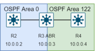
A regular area is just a non-backbone (nonzero) area without specific feature, generating and receiving summary and external LSAs. The backbone area is a special type of such area.
Stub area[edit]
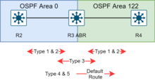
- In hello packets the E-flag is not high, indicating «External routing: not capable»
A stub area is an area that does not receive route advertisements external to the AS and routing from within the area is based entirely on a default route. An ABR deletes type 4 and 5 LSAs from internal routers, sends them a default route of 0.0.0.0 and turns itself into a default gateway. This reduces LSDB and routing table size for internal routers.
Modifications to the basic concept of stub area have been implemented by systems vendors, such as the totally stubby area (TSA) and the not-so-stubby area (NSSA), both an extension in Cisco Systems routing equipment.
Totally stubby area[edit]
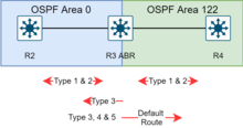
A totally stubby area is similar to a stub area. However, this area does not allow summary routes in addition to not having external routes, that is, inter-area (IA) routes are not summarized into totally stubby areas. The only way for traffic to get routed outside the area is a default route which is the only Type-3 LSA advertised into the area. When there is only one route out of the area, fewer routing decisions have to be made by the route processor, which lowers system resource utilization.
- Occasionally, it is said that a TSA can have only one ABR.[20]
Not-so-stubby area[edit]

- In hello packets the N-flag is set high, indicating «NSSA: supported»
A not-so-stubby area (NSSA) is a type of stub area that can import autonomous system external routes and send them to other areas, but still cannot receive AS-external routes from other areas.[21]
NSSA is an extension of the stub area feature that allows the injection of external routes in a limited fashion into the stub area. A case study simulates an NSSA getting around the stub-area problem of not being able to import external addresses. It visualizes the following activities: the ASBR imports external addresses with a type 7 LSA, the ABR converts a type 7 LSA to type 5 and floods it to other areas, the ABR acts as an «ASBR» for other areas.
The ASBRs do not take type 5 LSAs and then convert to type 7 LSAs for the area.
Totally not-so-stubby area[edit]

An addition to the standard functionality of an NSSA, the totally stubby NSSA is an NSSA that takes on the attributes of a TSA, meaning that type 3 and 4 summary routes are not flooded into this type of area. It is also possible to declare an area both totally stubby and not-so-stubby, which means that the area will receive only the default route from area 0.0.0.0, but can also contain an autonomous system boundary router (ASBR) that accepts external routing information and injects it into the local area, and from the local area into area 0.0.0.0.
- Redistribution into an NSSA area creates a special type of LSA known as type 7, which can exist only in an NSSA area. An NSSA ASBR generates this LSA, and an NSSA ABR router translates it into a type 5 LSA, which gets propagated into the OSPF domain.
A newly acquired subsidiary is one example of where it might be suitable for an area to be simultaneously not-so-stubby and totally stubby if the practical place to put an ASBR is on the edge of a totally stubby area. In such a case, the ASBR does send externals into the totally stubby area, and they are available to OSPF speakers within that area. In Cisco’s implementation, the external routes can be summarized before injecting them into the totally stubby area. In general, the ASBR should not advertise default into the TSA-NSSA, although this can work with extremely careful design and operation, for the limited special cases in which such an advertisement makes sense.
By declaring the totally stubby area as NSSA, no external routes from the backbone, except the default route, enter the area being discussed. The externals do reach area 0.0.0.0 via the TSA-NSSA, but no routes other than the default route enter the TSA-NSSA. Routers in the TSA-NSSA send all traffic to the ABR, except to routes advertised by the ASBR.
Router types[edit]
OSPF defines the following overlapping categories of routers:
- Internal router (IR)
- An internal router has all its interfaces belonging to the same area.
- Area border router (ABR)
- An area border router is a router that connects one or more areas to the main backbone network. It is considered a member of all areas it is connected to. An ABR keeps multiple instances of the link-state database in memory, one for each area to which that router is connected.
- Backbone router (BR)
- A backbone router has an interface to the backbone area. Backbone routers may also be area routers, but do not have to be.
- Autonomous system boundary router (ASBR)
- An autonomous system boundary router is a router that is connected by using more than one routing protocol and that exchanges routing information with routers autonomous systems. ASBRs typically also run an exterior routing protocol (e.g., BGP), or use static routes, or both. An ASBR is used to distribute routes received from other, external ASs throughout its own autonomous system. An ASBR creates External LSAs for external addresses and floods them to all areas via ABR. Routers in other areas use ABRs as next hops to access external addresses. Then ABRs forward packets to the ASBR that announces the external addresses.
The router type is an attribute of an OSPF process. A given physical router may have one or more OSPF processes. For example, a router that is connected to more than one area, and which receives routes from a BGP process connected to another AS, is both an area border router and an autonomous system boundary router.
Each router has an identifier, customarily written in the dotted-decimal format (e.g., 1.2.3.4) of an IP address. This identifier must be established in every OSPF instance. If not explicitly configured, the highest logical IP address will be duplicated as the router identifier. However, since the router identifier is not an IP address, it does not have to be a part of any routable subnet in the network, and often isn’t to avoid confusion.
Non-point-to-point network[edit]

On networks (same subnet) with networks type of:
- Broadcast
- Non-Broadcast Multi-Access (NBMA)
A system of designated router (DR) and backup designated router (BDR), is used to reducing network traffic by providing a source for routing updates.
This is done using multicast addresses:
- 224.0.0.5, all routers in the topology will listen on that multicast address.
- 224.0.0.6, DR and BDR will listen on that multicast address.
The DR and BDR maintains a complete topology table of the network and sends the updates to the other routers via multicast. All routers in a multi-access network segment will form a leader/follower relationship with the DR and BDR. They will form adjacencies with the DR and BDR only. Every time a router sends an update, it sends it to the DR and BDR on the multicast address 224.0.0.6. The DR will then send the update out to all other routers in the area, to the multicast address 224.0.0.5. This way all the routers do not have to constantly update each other, and can rather get all their updates from a single source. The use of multicasting further reduces the network load. DRs and BDRs are always setup/elected on OSPF broadcast networks. DR’s can also be elected on NBMA (Non-Broadcast Multi-Access) networks such as Frame Relay or ATM. DRs or BDRs are not elected on point-to-point links (such as a point-to-point WAN connection) because the two routers on either side of the link must become fully adjacent and the bandwidth between them cannot be further optimized. DR and non-DR routers evolve from 2-way to full adjacency relationships by exchanging DD, Request, and Update.
Designated router[edit]
A designated router (DR) is the router interface elected among all routers on a particular multiaccess network segment, generally assumed to be broadcast multiaccess. Special techniques, often vendor-dependent, may be needed to support the DR function on non-broadcast multiaccess (NBMA) media. It is usually wise to configure the individual virtual circuits of an NBMA subnet as individual point-to-point lines; the techniques used are implementation-dependent.
Backup designated router[edit]
A backup designated router (BDR) is a router that becomes the designated router if the current designated router has a problem or fails. The BDR is the OSPF router with the second-highest priority at the time of the last election.
A given router can have some interfaces that are designated (DR) and others that are backup designated (BDR), and others that are non-designated. If no router is a DR or a BDR on a given subnet, the BDR is first elected, and then a second election is held for the DR.[1]: 75
DR Other[edit]
A router that has not been selected to be designated router (DR) or backup designated router (BDR). The router forms an adjacency to both the designated router (DR) and the backup designated router (BDR).
For other non (B)DR, the adjacency stops at 2-ways State.
Designated router election[edit]
The DR is elected based on the following default criteria:
- If the priority setting on an OSPF router is set to 0, that means it can NEVER become a DR or BDR.
- If no DR exists on the network, routes will wait until Wait Timer runs out.
- When a DR fails and the BDR takes over, there is another election to see who becomes the replacement BDR.
- The router sending the Hello packets with the highest priority wins the election.
- If two or more routers tie with the highest priority setting, the router sending the Hello with the highest RID (Router ID) wins. NOTE: a RID is the highest logical (loopback) IP address configured on a router, if no logical/loopback IP address is set then the router uses the highest IP address configured on its active interfaces (e.g. 192.168.0.1 would be higher than 10.1.1.2).
- Usually the router with the second-highest priority number becomes the BDR.
- The priority values range between 0 – 255,[22] with a higher value increasing its chances of becoming DR or BDR.
- If a higher priority OSPF router comes online after the election has taken place, it will not become DR or BDR until (at least) the DR and BDR fail.
- If the current DR ‘goes down’ the current BDR becomes the new DR and a new election takes place to find another BDR. If the new DR then ‘goes down’ and the original DR is now available, still previously chosen BDR will become DR.
Routing update flow[edit]
When DR has Routing update[edit]
- DR sends LSU to 224.0.0.5
- BDR sends LSUAck to 224.0.0.5
- DR Other sends LSUAck to 224.0.0.6
When BDR has Routing update[edit]
- BDR sends LSU to 224.0.0.5
- BDR sends LSUAck to 224.0.0.5
- DR Other sends LSUAck to 224.0.0.6
When DR Other has Routing update[edit]
- DR Other sends LSU to 224.0.0.6
- BDR sends LSA to 224.0.0.5
- BDR sends LSUAck to 224.0.0.5
- Non-source routers, DR Other sends LSUAck to 224.0.0.6
Protocol messages[edit]
| 1 | 1 | 2 | 4 | 4 | 2 | 2 | 8 | Variable |
|---|---|---|---|---|---|---|---|---|
| Header 24 byte | Data | |||||||
| Version 2 | Type | Packet length | Router ID | Area ID | Checksum | AuType | Authentication |
| 1 | 1 | 2 | 4 | 4 | 2 | 1 | 1 | Variable |
|---|---|---|---|---|---|---|---|---|
| Header 16 byte | Data | |||||||
| Version 3 | Type | Packet length | Router ID | Area ID | Checksum | Instance ID | Reserved |
| 1 | 1 | 2 | 4 | 4 | 2 | 2 | 8 | Variable |
|---|---|---|---|---|---|---|---|---|
| Header 24 Byte | Data | |||||||
| Version #2 | Type | Packet length | Router ID | Area ID | Checksum | AuType | Authentication |
| 1 | 1 | 2 | 4 | 4 | 2 | 1 | 1 | Variable |
|---|---|---|---|---|---|---|---|---|
| Header 16 Byte | Data | |||||||
| Version #3 | Type | Packet length | Router ID | Area ID | Checksum | Instance ID | reserved |
Unlike other routing protocols, OSPF does not carry data via a transport protocol, such as the User Datagram Protocol (UDP) or the Transmission Control Protocol (TCP). Instead, OSPF forms IP datagrams directly, packaging them using protocol number 89 for the IP Protocol field. OSPF defines five different message types, for various types of communication. Multiple packets can be sent per frame.
OSPF uses the following packets 5 type:
- Hello
- Database description
- Link state request
- Link state update
- Link state acknowledgement
Hello Packet[edit]
| 24 | 4 | 2 | 1 | 1 | 4 | 4 | 4 | 4 |
|---|---|---|---|---|---|---|---|---|
| Header | ||||||||
| Network Mask | Hello Interval | Options | Router Priority | Router Dead Interval | Designated Router ID | Backup Designated Router ID | Neighbor ID |
| 16 | 4 | 1 | 3 | 2 | 2 | 4 | 4 | 4 |
|---|---|---|---|---|---|---|---|---|
| Header | ||||||||
| Interface ID | Router Priority | Options | Hello Interval | Router Dead Interval | Designated Router ID | Backup Designated Router ID | Neighbor ID |
OSPF’s Hello messages are used as a form of greeting, to allow a router to discover other adjacent routers on its local links and networks. The messages establish relationships between neighboring devices (called adjacencies) and communicate key parameters about how OSPF is to be used in the autonomous system or area. During normal operation, routers send hello messages to their neighbors at regular intervals (the hello interval); if a router stops receiving hello messages from a neighbor, after a set period (the dead interval) the router will assume the neighbor has gone down.
Database description (DBD)[edit]
| 16 or 24 | 2 | 1 | 1 | 1 | 4 | Variable |
|---|---|---|---|---|---|---|
| Header | ||||||
| Interface MTU | Hello Interval | Options | Flags | DD sequence number | LSA Headers |
Database description messages contain descriptions of the topology of the autonomous system or area. They convey the contents of the link-state database (LSDB) for the area from one router to another. Communicating a large LSDB may require several messages to be sent by having the sending device designated as a leader device and sending messages in sequence, with the follower (recipient of the LSDB information) responding with acknowledgments.
Link state packets[edit]
| 24 | 4 | 4 | 4 |
|---|---|---|---|
| Header | |||
| LS Type | Link State ID | Advertising Router |
| 16 | 2 | 2 | 4 | 4 |
|---|---|---|---|---|
| Header | ||||
| 0’s | LS Type | Link State ID | Advertising Router |
- Link state request (LSR)
- Link state request messages are used by one router to request updated information about a portion of the LSDB from another router. The message specifies the link(s) for which the requesting device wants more current information.
| 24 or 16 | 4 | 4- |
|---|---|---|
| Header | ||
| # LSAs | list of LSAs |
- Link state update (LSU)
- Link-state update messages contain updated information about the state of certain links on the LSDB. They are sent in response to a link state request message, and also broadcast or multicast by routers on a regular basis. Their contents are used to update the information in the LSDBs of routers that receive them.
| 24 or 16 | 4- |
|---|---|
| Header | |
| list of LSAs |
- Link state acknowledgment (LSAck)
- Link-state acknowledgment messages provide reliability to the link-state exchange process, by explicitly acknowledging receipt of a Link State Update message.
| LS type | LS name | Generated by | Description |
|---|---|---|---|
| 1 | Router-LSAs | Each internal router within an area | 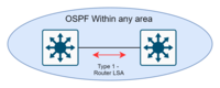 The link-state ID of the type 1 LSA is the originating router ID.
|
| 2 | Network-LSAs | The DR |  |
| 3 | Summary-LSAs | The ABR |  To inform other areas about inter-area routers. These routes can also be summarised. |
| 4 | ASBR-summary | The ABR | Type 4 describe routes to AS boundary routers beyond its area.
The area border router (ABR) generates this LSA to inform other routers in the OSPF domain, that the matching router is an autonomous system boundary router (ASBR), so that the external LSAs (Type 5 / Type 7) it sent may be properly resolved outside its own area. |
| 5 | AS-external-LSAs | The ASBR |  LSAs contain information imported into OSPF from other routing processes. Together with Type 4 they describe they way to an external route. |
| 7 | NSSA external link-state advertisements | The ASBR, within a not-so-stubby area | Type 7-LSAs are identical to type-5 LSAs. Type-7 LSAs are only flooded within the NSSA. At the area border router, selected type-7 LSAs are translated into type 5-LSAs and flooded into the backbone. |
| 8 | Link-LSA (v3) | Each internal router within a link | Provide it local router’s link-local address to all other routers on the local network. |
| 9 | Intra-Area-Prefix-LSAs (v3) | Each internal router within an area | Replaces some of the functionality of Router-LSAs; stub network segment, or an attached transit network segment. |
OSPF v2 area types and accepted LSAs[edit]
Not all area types use all LSA. Below is a matrix of accepted LSAs.
| Within a single area | Inter area | |||||
|---|---|---|---|---|---|---|
| Area type | LSA 1 — router | LSA 2 — network | LSA 7 — NSSA external | LSA 3 — network summary | LSA 4 — ASBR Summary | LSA 5 — AS external |
| Backbone | Yes | Yes | No, converted into a Type 5 by the ABR | Yes | Yes | Yes |
| Non-backbone | Yes | Yes | No, converted into a Type 5 by the ABR | Yes | Yes | Yes |
| Stub | Yes | Yes | No, Default route | Yes | No, Default route | No, Default route |
| Totally stubby | Yes | Yes | No, Default route | No, Default route | No, Default route | No, Default route |
| Not-so-stubby | Yes | Yes | Yes | Yes | No, Default route | No, Default route |
| Totally not-so-stubby | Yes | Yes | Yes | No, Default route | No, Default route | No, Default route |
Routing metrics[edit]
OSPF uses path cost as its basic routing metric, which was defined by the standard not to equate to any standard value such as speed, so the network designer could pick a metric important to the design. In practice, it is determined by comparing the speed of the interface to a reference-bandwidth for the OSPF process. The cost is determined by dividing the reference bandwidth by the interface speed (although the cost for any interface can be manually overridden). If a reference bandwidth is set to ‘10000’, then a 10 Gbit/s link will have a cost of 1. Any speeds less than 1 are rounded up to 1.[25] Here is an example table that shows the routing metric or ‘cost calculation’ on an interface.
- Type-1 LSA has a size of 16-bit field (65,535 in decimal)[26]
- Type-3 LSA has a size of 24-bit field (16,777,216 in decimal)
| Interface speed | Link cost | Uses | |
|---|---|---|---|
| Default (100 Mbit/s) | 200 Gbit/s | ||
| 800 Gbit/s | 1 | 1 | QSFP-DD112 |
| 200 Gbit/s | 1 | 1 | SFP-DD |
| 40 Gbit/s | 1 | 5 | QSFP+ |
| 25 Gbit/s | 1 | 8 | SFP28 |
| 10 Gbit/s | 1 | 20 | 10 GigE, common in data centers |
| 5 Gbit/s | 1 | 40 | NBase-T, Wi-Fi routers |
| 1 Gbit/s | 1 | 200 | common gigabit port |
| 100 Mbit/s | 1 | 2000 | low-end port |
| 10 Mbit/s | 10 | 20000 | 1990’s speed. |
OSPF is a layer 3 protocol. If a layer 2 switch is between the two devices running OSPF, one side may negotiate a speed different from the other side. This can create an asymmetric routing on the link (Router 1 to Router 2 could cost ‘1’ and the return path could cost ’10’), which may lead to unintended consequences.
Metrics, however, are only directly comparable when of the same type. Four types of metrics are recognized. In decreasing preference (for example, an intra-area route is always preferred to an external route regardless of metric), these types are:
- Intra-area
- Inter-area
- External Type 1, which includes both the external path cost and the sum of internal path costs to the ASBR that advertises the route,[27]
- External Type 2, the value of which is solely that of the external path cost,
OSPF v3[edit]
OSPF version 3 introduces modifications to the IPv4 implementation of the protocol.[2]
Despite the expansion of addresses to 128 bits in IPv6, area and router identifications are still 32-bit numbers.
High-level changes[edit]
- Except for virtual links, all neighbor exchanges use IPv6 link-local addressing exclusively. The IPv6 protocol runs per link, rather than based on the subnet.
- All IP prefix information has been removed from the link-state advertisements and from the hello discovery packet, making OSPFv3 essentially protocol-independent.
- Three separate flooding scopes for LSAs:
- Link-local scope: LSA is flooded only on the local link and no further.
- Area scope: LSA is flooded throughout a single OSPF area.
- AS scope: LSA is flooded throughout the routing domain.
- Use of IPv6 link-local addresses, for neighbor discovery, auto-configuration.
- Authentication has been moved to the IP Authentication Header
Changes introduced in OSPF v3, then backported by vendors to v2[edit]
- Explicit support for multiple instances per link[28]
Packet format changes[edit]
- OSPF version number changed to 3
- From the LSA header, the options field has been removed.
- In hello packets and database description, the options field is changed from 16 to 24 bits.
- In hello packet, the address information has been removed. The interface ID has been added.
- In router-LSAs, two options bits, the «R-bit» and the «V6-bit», have been added.
- «R-bit»: allows for multi-homed hosts to participate in the routing protocol.
- «V6-bit»: specializes the R-bit.
- Add «instance ID», which allows multiple OSPF protocol instances on the same logical interface.
LSA format changes[edit]
- The LSA type field is changed to 16 bits.
- Add support for handling unknown LSA types
- Three bits are used for encoding flooding scope.
- With IPv6, addresses in LSAs are expressed as prefix and prefix length.
- In router-LSAs and network-LSAs, the address information is removed.
- Router-LSAs and network-LSAs are made network-protocol independent.
- A new LSA type is added, link-LSA, which provides the router’s link-local address to all other routers attached to the logical interface, provides a list of IPv6 prefixes to associate with the link, and can send information that reflect the router’s capabilities.
- LSA Type-3 summary-LSAs have been renamed «inter-area-prefix-LSAs».
- LSA Type-4 summary LSAs have been renamed «inter-area-router-LSAs».
- Intra-area-prefix-LSA is added, an LSA that carries all IPv6 prefix information.
OSPF over MPLS-VPN[edit]
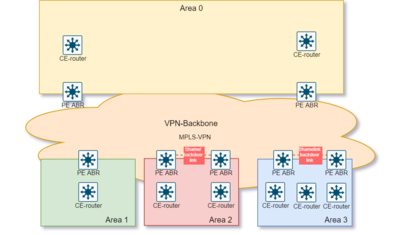
| Type | Type field | sub value | name |
|---|---|---|---|
| Two-octet AS | 0x00 | 0x05 | OSPF domain identifier |
| Four-octet AS | 0x02 | 0x05 | OSPF domain identifier |
| IPv4 address | 0x01 | 0x05 | OSPF domain identifier |
| IPv4 address | 0x01 | 0x07 | OSPF route ID |
| Opaque | 0x03 | 0x06 | OSPF route type |
| 4 byte | 1 byte | 1 byte |
|---|---|---|
| Area number | Route type | Options |
A customer can use OSPF over a MPLS-VPN, where the service provider uses BGP or RIP as their interior gateway protocol.[30]
When using OSPF over MPLS-VPN, the VPN backbone becomes part of the OSPF backbone area 0. In all areas, isolated copies of the IGP are run.
Advantages:
- The MPLS-VPN is transparent to the customer’s OSPF standard routing.
- Customer’s equipment only needs to support OSPF.
- Reduce the need for tunnels (Generic Routing Encapsulation, IPsec, wireguard) to use OSPF.
To achieve this, a non-standard OSPF-BGP redistribution is used. All OSPF routes retain the source LSA type and metric.[31][32]
To prevent loops, an optional DN bit[33] is used in LSAs to indicate that a route has already been sent from the provider edge to the customer’s equipment.
OSPF extensions[edit]
Traffic engineering[edit]
OSPF-TE is an extension to OSPF extending the expressivity to allow for traffic engineering and use on non-IP networks.[34] Using OSPF-TE, more information about the topology can be exchanged using opaque LSA carrying type–length–value elements. These extensions allow OSPF-TE to run completely out of band of the data plane network. This means that it can also be used on non-IP networks, such as optical networks.
OSPF-TE is used in GMPLS networks as a means to describe the topology over which GMPLS paths can be established. GMPLS uses its own path setup and forwarding protocols, once it has the full network map.
In the Resource Reservation Protocol (RSVP), OSPF-TE is used for recording and flooding RSVP signaled bandwidth reservations for label-switched paths within the link-state database.
Optical routing[edit]
RFC 3717 documents work in optical routing for IP based on extensions to OSPF and IS-IS.[35]
Multicast Open Shortest Path First[edit]
The Multicast Open Shortest Path First (MOSPF) protocol is an extension to OSPF to support multicast routing. MOSPF allows routers to share information about group memberships.
Notable implementations[edit]
- Allied Telesis implements OSPFv2 & OSPFv3 in Allied Ware Plus (AW+)
- Arista Networks implements OSPFv2 and OSPFv3
- BIRD implements both OSPFv2 and OSPFv3
- Cisco IOS and NX-OS
- Cisco Meraki
- D-Link implements OSPFv2 on Unified Services Router.
- Dell’s FTOS implements OSPFv2 and OSPFv3
- ExtremeXOS
- FRRouting, the successor of Quagga
- GNU Zebra, a GPL routing suite for Unix-like systems
- Juniper Junos
- NetWare implements OSPF in its Multi Protocol Routing module.
- OpenBSD includes OpenOSPFD, an OSPFv2 implementation.
- Quagga, a fork of GNU Zebra for Unix-like systems
- Windows NT 4.0 Server, Windows 2000 Server and Windows Server 2003 implemented OSPFv2 in the Routing and Remote Access Service, although the functionality was removed in Windows Server 2008.
- XORP, a routing suite implementing RFC2328 (OSPFv2) and RFC2740 (OSPFv3) for both IPv4 and IPv6
Applications[edit]
OSPF is a widely deployed routing protocol that can converge a network in a few seconds and guarantee loop-free paths. It has many features that allow the imposition of policies about the propagation of routes that it may be appropriate to keep local, for load sharing, and for selective route importing. IS-IS, in contrast, can be tuned for lower overhead in a stable network, the sort more common in ISP than enterprise networks. There are some historical accidents that made IS-IS the preferred IGP for ISPs, but ISPs today may well choose to use the features of the now-efficient implementations of OSPF,[36] after first considering the pros and cons of IS-IS in service provider environments.[37]
OSPF can provide better load-sharing on external links than other IGPs.[citation needed] When the default route to an ISP is injected into OSPF from multiple ASBRs as a Type I external route and the same external cost specified, other routers will go to the ASBR with the least path cost from its location. This can be tuned further by adjusting the external cost. If the default route from different ISPs is injected with different external costs, as a Type II external route, the lower-cost default becomes the primary exit and the higher-cost becomes the backup only.
See also[edit]
- Fabric Shortest Path First
- Mesh networking
- Route analytics
- Routing
- Shortest path problem
References[edit]
- ^ a b c d J. Moy (April 1998). OSPF Version 2. Network Working Group, IETF. doi:10.17487/RFC2328. OSPFv2., Updated by RFC 5709, RFC 6549, RFC 6845, RFC 6860, RFC 7474, RFC 8042.
- ^ a b c R. Coltun; D. Ferguson; J. Moy (July 2008). A. Lindem (ed.). OSPF for IPv6. Network Working Group, IETF. doi:10.17487/RFC5340. OSPFv3. Updated by RFC 6845, RFC 6860, RFC 7503, RFC 8362.
- ^ OSPF Convergence, August 6, 2009, retrieved June 13, 2016
- ^ Moy, J. (April 2, 1998). «RFC 2328 — OSPF Version 2». Tools.ietf.org. doi:10.17487/RFC2328. Retrieved November 30, 2011.
- ^ Coltun, R.; Ferguson, D.; Moy, J.; Lindem, A. (2008). «RFC 5340 — OSPF for IPv6». Tools.ietf.org. doi:10.17487/RFC5340. Retrieved November 30, 2011.
- ^ RFC 1584, Multicast Extensions to OSPF, J. Moy, The Internet Society (March 1994)
- ^ IP Routing: OSPF Configuration Guide, Cisco Systems, retrieved June 13, 2016,
Cisco routers do not support LSA Type 6 Multicast OSPF (MOSPF), and they generate syslog messages if they receive such packets.
- ^ «[Junos] GRE Configuration Example — Juniper Networks». kb.juniper.net. Retrieved November 28, 2021.
- ^ «Generic Routing Encapsulation (GRE) | Interfaces User Guide for Switches | Juniper Networks TechLibrary». www.juniper.net. Retrieved November 28, 2021.
- ^ Eric C. Rosen; Peter Psenak; Padma Pillay-Esnault (June 2006). OSPF as the Provider/Customer Edge Protocol for BGP/MPLS IP Virtual Private Networks (VPNs). Internet Engineering Task Force. doi:10.17487/RFC4577. RFC 4577.
- ^ «Understanding OSPF Sham Links — Technical Documentation — Support — Juniper Networks». www.juniper.net. Retrieved November 14, 2021.
- ^ «IP Routing: OSPF Configuration Guide, Cisco IOS Release 15SY — OSPF Sham-Link Support for MPLS VPN [Cisco IOS 15.1SY]». Cisco. Retrieved November 14, 2021.
- ^ «OSPF Neighbor States». Cisco. Retrieved October 28, 2018.
- ^ «Show 134 – OSPF Design Part 1 – Debunking the Multiple Area Myth». Packet Pushers. podcast debunking 50-router advice on old Cisco article
- ^ Mikrotik RB4011 has 1 GB RAM for example, mikrotik.com, Retrieved Feb 1, 2021.
- ^ «Stub Area Design Golden Rules». Groupstudy.com. Archived from the original on August 31, 2000. Retrieved November 30, 2011. 64 MB of RAM was a big deal in 2020 for OSPF.
- ^ Doyle, Jeff (September 10, 2007). «My Favorite Interview Question». Network World. Retrieved December 28, 2021.
- ^ (ASGuidelines 1996, p. 25)
- ^ Hawkinson, J; T. Bates (March 1996). «Guidelines for creation, selection, and registration of an Autonomous System». Internet Engineering Task Force. doi:10.17487/RFC1930. ASguidelines. Retrieved September 28, 2007.
- ^ «Stub Area Design Golden Rules». Groupstudy.com. Archived from the original on August 31, 2000. Retrieved November 30, 2011.. This is not necessarily true. If there are multiple ABRs, as might be required for high availability, routers interior to the TSA will send non-intra-area traffic to the ABR with the lowest intra-area metric (the «closest» ABR) but that requires special configuration.
- ^ Murphy, P. (January 2003). «The OSPF Not-So-Stubby Area (NSSA) Option». The Internet Society. doi:10.17487/RFC3101. Retrieved June 22, 2014.
- ^ «Cisco IOS IP Routing: OSPF Command Reference» (PDF). Cisco Systems. April 2011. Archived from the original (PDF) on April 25, 2012.
- ^ «juniper configuring-ospf-areas». Juniper Networks. January 18, 2021. Retrieved October 23, 2021.
- ^ «OSPF Area’s Explained». Packet Coders. January 23, 2019. Retrieved October 23, 2021.
- ^ Adjusting OSPF Costs, OReilly.com
- ^ «OSPF Stub Router Advertisement». Ietf Datatracker. Internet Engineering Task Force. June 2001. Retrieved October 23, 2021.
- ^ Whether an external route is based on a Type-5 LSA or a Type-7 LSA (NSSA) does not affect its preference. See RFC 3101, section 2.5.
- ^ «secondary (Protocols OSPF) — TechLibrary — Juniper Networks». www.juniper.net. Retrieved November 7, 2021.
- ^ «Border Gateway Protocol (BGP) Extended Communities». www.iana.org. Retrieved November 28, 2021.
- ^ RFC 4577
- ^ «MPLS VPN OSPF PE and CE Support». Cisco. Retrieved November 28, 2021.
- ^ Cisco. «Using OSPF in an MPLS VPN Environment» (PDF). Archived (PDF) from the original on October 10, 2022. Retrieved November 28, 2021.
- ^ RFC 4576
- ^ Katz, D; D. Yeung (September 2003). Traffic Engineering (TE) Extensions to OSPF Version 2. The Internet Society. doi:10.17487/RFC3630. OSPF-TEextensions. Retrieved September 28, 2007.
- ^ B. Rajagopalan; J. Luciani; D. Awduche (March 2004). IP over Optical Networks: A Framework. Internet Engineering Task Force. doi:10.17487/RFC3717. RFC 3717.
- ^ Berkowitz, Howard (1999). OSPF Goodies for ISPs. North American Network Operators Group NANOG 17. Montreal. Archived from the original on June 12, 2016.
- ^ Katz, Dave (2000). OSPF and IS-IS: A Comparative Anatomy. North American Network Operators Group NANOG 19. Albuquerque. Archived from the original on June 20, 2018.
Further reading[edit]
- Colton, Andrew (October 2003). OSPF for Cisco Routers. Rocket Science Press. ISBN 978-0972286213.
- Doyle, Jeff; Carroll, Jennifer (2005). Routing TCP/IP. Vol. 1 (2nd ed.). Cisco Press. ISBN 978-1-58705-202-6.
- Moy, John T. (1998). OSPF: Anatomy of an Internet Routing Protocol. Addison-Wesley. ISBN 978-0201634723.
- Parkhurst, William R. (2002). Cisco OSPF Command and Configuration Handbook. ISBN 978-1-58705-071-8.
- Basu, Anindya; Riecke, Jon (2001). «Stability issues in OSPF routing». Proceedings of the 2001 conference on Applications, technologies, architectures, and protocols for computer communications. SIGCOMM ’01. pp. 225–236. CiteSeerX 10.1.1.99.6393. doi:10.1145/383059.383077. ISBN 978-1-58113-411-7. S2CID 7555753.
- Valadas, Rui (2019). OSPF and IS-IS: From Link State Routing Principles to Technologies. CRC Press. doi:10.1201/9780429027543. ISBN 9780429027543. S2CID 164731068.
External links[edit]
- IETF OSPF Working Group
- Cisco OSPF
- Cisco OSPF Areas and Virtual Links
- Summary of OSPF v2
Overview
OSPF is Interior Gateway Protocol (IGP) designed to distribute routing information between routers belonging to the same Autonomous System (AS).
The protocol is based on link-state technology that has several advantages over distance-vector protocols such as RIP:
- no hop count limitations;
- multicast addressing is used to send routing information updates;
- updates are sent only when network topology changes occur;
- the logical definition of networks where routers are divided into areas
- transfers and tags external routes injected into AS.
However, there are a few disadvantages:
- OSPF is quite CPU and memory intensive due to the SPF algorithm and maintenance of multiple copies of routing information;
- more complex protocol to implement compared to RIP;
RouterOS implements the following standards:
- RFC 2328 — OSPF Version 2
- RFC 3101 — The OSPF Not-So-Stubby Area (NSSA) Option
- RFC 3630 — Traffic Engineering (TE) Extensions to OSPF Version 2
- RFC 4577 — OSPF as the Provider/Customer Edge Protocol for BGP/MPLS IP Virtual Private Networks (VPNs)
- RFC 5329 — Traffic Engineering Extensions to OSPF Version 3
- RFC 5340 — OSPF for IPv6
- RFC 5643 — Management Information Base for OSPFv3
- RFC 6549 — OSPFv2 Multi-Instance Extensions
- RFC 6565 — OSPFv3 as a Provider Edge to Customer Edge (PE-CE) Routing Protocol
- RFC 6845 — OSPF Hybrid Broadcast and Point-to-Multipoint Interface Type
- RFC 7471 — OSPF Traffic Engineering (TE) Metric Extensions
OSPF Terminology
Before we move on let’s familiarise ourselves with terms important for understanding the operation of the OSPF. These terms will be used throughout the article.
- Neighbor — connected (adjacent) router that is running OSPF with the adjacent interface assigned to the same area. Neighbors are found by Hello packets (unless manually configured).
- Adjacency — logical connection between a router and its corresponding DR and BDR. No routing information is exchanged unless adjacencies are formed.
- Link — link refers to a network or router interface assigned to any given network.
- Interface — physical interface on the router. The interface is considered a link when it is added to OSPF. Used to build link database.
- LSA — Link State Advertisement, data packet contains link-state and routing information, that is shared among OSPF Neighbors.
- DR — Designated Router, chosen router to minimize the number of adjacencies formed. The option is used in broadcast networks.
- BDR -Backup Designated Router, hot standby for the DR. BDR receives all routing updates from adjacent routers, but it does not flood LSA updates.
- Area — areas are used to establish a hierarchical network.
- ABR — Area Border Router, router connected to multiple areas. ABRs are responsible for summarization and update suppression between connected areas.
- ASBR — Autonomous System Boundary Router, router connected to an external network (in a different AS). If you import other protocol routes into OSPF from the router it is now considered ASBR.
- NBMA — Non-broadcast multi-access, networks allow multi-access but have no broadcast capability. Additional OSPF neighbor configuration is required for those networks.
- Broadcast — Network that allows broadcasting, for example, Ethernet.
- Point-to-point — Network type eliminates the need for DRs and BDRs
- Router-ID — IP address used to identify the OSPF router. If the OSPF Router-ID is not configured manually, a router uses one of the IP addresses assigned to the router as its Router-ID.
- Link State — The term link-state refers to the status of a link between two routers. It defines the relationship between a router’s interface and its neighboring routers.
- Cost — Link-state protocols assign a value to each link called cost. the cost value depends on the speed of the media. A cost is associated with the outside of each router interface. This is referred to as interface output cost.
- Autonomous System — An autonomous system is a group of routers that use a common routing protocol to exchange routing information.
Basic Configuration Example
To start OSPF v2 and v3 instances, the first thing to do is to add the instance and the backbone area:
/routing ospf instance
add name=v2inst version=2 router-id=1.2.3.4
add name=v3inst version=3 router-id=1.2.3.4
/routing ospf area
add name=backbone_v2 area-id=0.0.0.0 instance=v2inst
add name=backbone_v3 area-id=0.0.0.0 instance=v3inst
At this point, we can add a template. The template is used to match interfaces on which OSPF should be running, it can be done either by specifying the network or interface directly.
/routing ospf interface-template
add networks=192.168.0.0/24 area=backbone_v2
add networks=2001:db8::/64 area=backbone_v3
add interfaces=ether1 area=backbone_v3
Routing Table Calculation
Link state database describes the routers and links that interconnect them and are appropriate for forwarding. It also contains the cost (metric) of each link. This metric is used to calculate the shortest path to the destination network.
Each router can advertise a different cost for the router’s own link direction, making it possible to have asymmetric links (packets to the destination travel over one path, but the response travels a different path). Asymmetric paths are not very popular, because it makes it harder to find routing problems.
The value of the cost can be changed in the OSPF interface template configuration menu, for example, to add an ether2 interface with a cost of 100:
/routing ospf interface-template
add interfaces=ether2 cost=100 area=backbone_v2
The cost of an interface on Cisco routers is inversely proportional to the bandwidth of that interface. A higher bandwidth indicates a lower cost. If similar costs are necessary on RouterOS, then use the following formula:
Cost = 100000000/bw in bps.
OSPF router is using Dijkstra’s Shortest Path First (SPF) algorithm to calculate the shortest path. The algorithm places the router at the root of a tree and calculates the shortest path to each destination based on the cumulative cost required to reach the destination. Each router calculates its own tree even though all routers are using the same link-state database.
SPT Calculation
Assume we have the following network. The network consists of 4(four) routers. OSPF costs for outgoing interfaces are shown near the line that represents the link. In order to build the shortest-path tree for router R1, we need to make R1 the root and calculate the smallest cost for each destination.
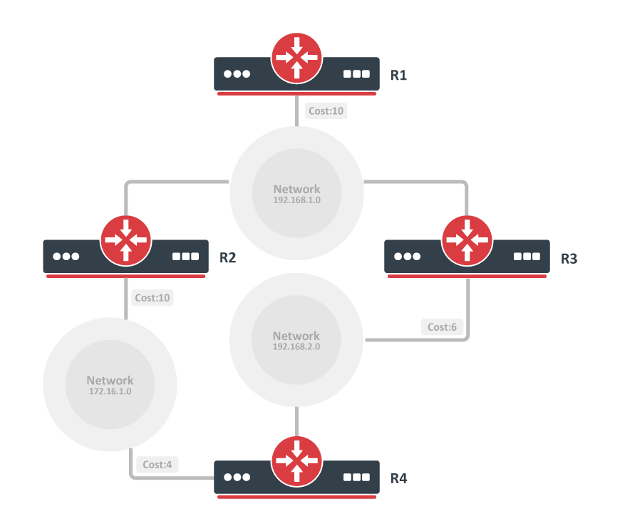
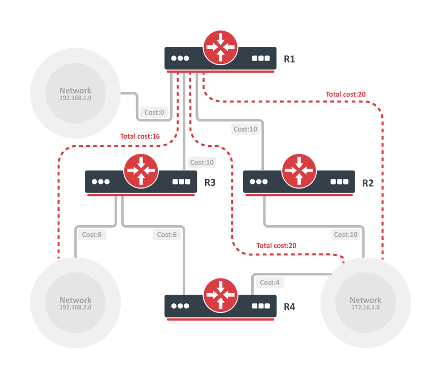
As you can see from the image above multiple shortest paths have been found to the 172.16.1.0 network, allowing load balancing of the traffic to that destination called equal-cost multipath (ECMP). After the shortest-path tree is built, a router starts to build the routing table accordingly. Networks are reached consequently to the cost calculated in the tree.
Routing table calculation looks quite simple, however, when some of the OSPF extensions are used or OSPF areas are calculated, routing calculation gets more complicated.
Forwarding Address
OSPF router can set the forwarding-address to something other than itself which indicates that an alternate next-hop is possible. Mostly forwarding address is set to 0.0.0.0 suggesting that the route is reachable only via the advertising router.
The forwarding address is set in LSA if the following conditions are met:
- OSPF must be enabled on the next-hop interface
- Next-hop address falls into the network provided by OSPF networks
A router that receives such LSA can use a forwarding address if OSPF is able to resolve the forwarding address. If forwarding address is not resolved directly — router sets nexthop for forwading address from LSA as a gateway, if forwarding address is not resolved at all — the gateway will be originator-id. Resolve happens only using OSPF instance routes, not the whole routing table.
Let’s look at the example setup below:
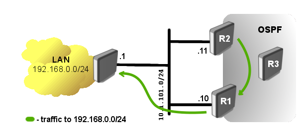
Router R1 has a static route to the external network 192.168.0.0/24. OSPF is running between R1, R2, and R3, and the static route is distributed across the OSPF network.
The problem in such a setup is obvious, R2 can not reach the external network directly. Traffic going to the LAN network from R2 will be forwarded over the router R1, but if we look at the network diagram we can see that more R2 can directly reach the router where the LAN network i located.
So knowing the forwarding address conditions, we can make router R1 to set the forwarding address. We simply need to add 10.1.101.0/24 network to OSPF networks in the router’s R1 configuration:
/routing/ospf/interface-template add area=backbone_v2 networks=10.1.101.0/24
Now lets verify that forwarding address is actually working:
[admin@r2] /ip/route> print where dst-address=192.168.0.0/24
Flags: D - DYNAMIC; A - ACTIVE; o, y - COPY
Columns: DST-ADDRESS, GATEWAY, DISTANCE
    DST-ADDRESS       GATEWAY            DISTANCE
DAo 192.168.0.0/24    10.1.101.1%ether1       110
On all OSPF routers you will see LSA set with forwarding address other than 0.0.0.0
[admin@r2] /routing/ospf/lsa> print where id=192.168.0.0
Flags: S - self-originated, F - flushing, W - wraparound; D - dynamic

 1  D instance=default_ip4 type="external" originator=10.1.101.10 id=192.168.0.0
      sequence=0x80000001 age=19 checksum=0xF336 body=
        options=E
        netmask=255.255.255.0
        forwarding-address=10.1.101.1
        metric=10 type-1
        route-tag=0
OSPF adjacency between routers in the 10.1.101.0/24 network is not required
Neighbour Relationship and Adjacency
OSPF is a link-state protocol that assumes that the interface of the router is considered an OSPF link. Whenever OSPF is started, it adds the state of all the links in the local link-state database.
There are several steps before the OSPF network becomes fully functional:
- Neighbors discovery
- Database Synchronization
- Routing calculation
Link-state routing protocols are distributing and replicating database that describes the routing topology. The link-state protocol’s flooding algorithm ensures that each router has an identical link-state database and the routing table is calculated based on this database.
After all the steps above are completed link-state database on each neighbor contains full routing domain topology (how many other routers are in the network, how many interfaces routers have, what networks link between router connects, cost of each link, and so on).
Communication Between OSPF Routers
OSPF operates over the IP network layer using protocol number 89.
A destination IP address is set to the neighbor’s IP address or to one of the OSPF multicast addresses AllSPFRouters (224.0.0.5) or AllDRRouters (224.0.0.6). The use of these addresses is described later in this article.
Every OSPF packet begins with a standard 24-byte header.
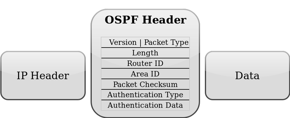
| Field | Description |
|---|---|
| Packet type | There are several types of OSPF packets: Hello packet, Database Description (DD) packet, Link state request packet, Link State Update packet, and Link State Acknowledgement packet. All of these packets except the Hello packet are used in link-state database synchronization. |
| Router ID | one of the router’s IP addresses unless configured manually |
| Area ID | Allows OSPF router to associate the packet to the proper OSPF area. |
| Checksum | Allows receiving router to determine if a packet was damaged in transit. |
| Authentication fields | These fields allow the receiving router to verify that the packet’s contents were not modified and that packet really came from the OSPF router whose Router ID appears in the packet. |
There are five different OSPF packet types used to ensure proper LSA flooding over the OSPF network.
- Hello packet — used to discover OSPF neighbors and build adjacencies.
- Database Description (DD) — check for Database synchronization between routers. Exchanged after adjacencies are built.
- Link-State Request (LSR) — used to request up-to-date pieces of the neighbor’s database. Out-of-date parts of the routing database are determined after the DD exchange.
- Link-State Update (LSU) — carries a collection of specifically requested link-state records.
- Link-State Acknowledgment (LSack) — is used to acknowledge other packet types that way introducing reliable communication.
Neighbors Discovery
OSPF discovers potential neighbors by periodically sending Hello packets out of configured interfaces. By default Hello packets are sent out at 10-second intervals which can be changed by setting hello-interval in OSPF interface settings. The router learns the existence of a neighboring router when it receives the neighbor’s Hello in return with matching parameters.
The transmission and reception of Hello packets also allow a router to detect the failure of the neighbor. If Hello packets are not received within dead-interval (which by default is 40 seconds) router starts to route packets around the failure. «Hello» protocol ensures that the neighboring routers agree on the Hello interval and Dead interval parameters, preventing situations when not in time received Hello packets mistakenly bring the link down.
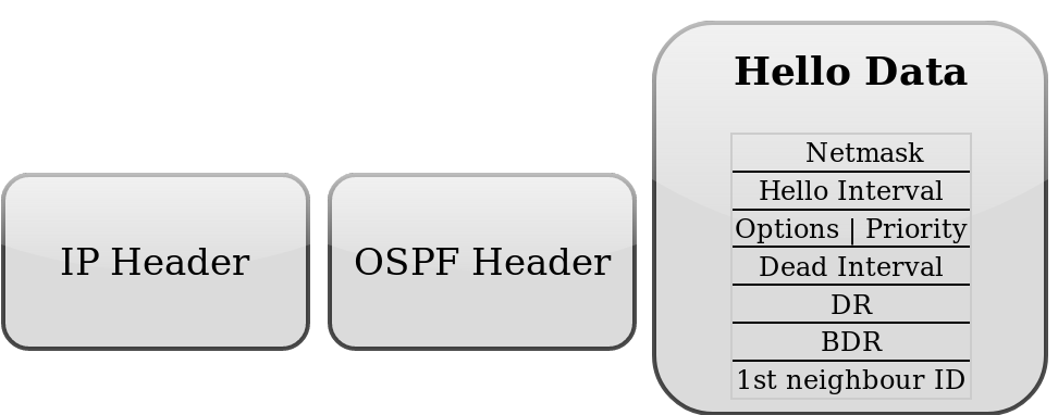
| Field | Description |
|---|---|
| network mask | The IP mask of the originating router’s interface IP address. |
| hello interval | the period between Hello packets (default 10s) |
| options | OSPF options for neighbor information |
| router priority | an 8-bit value used to aid in the election of the DR and BDR. (Not set in p2p links) |
| router dead interval | time interval has to be received before considering the neighbor is down. ( By default four times bigger than the Hello interval) |
| DR | the router-id of the current DR |
| BDR | the router-id of the current BDR |
| Neighbor router IDs | a list of router ids for all the originating router’s neighbors |
On each type of network segment Hello protocol works a little differently. It is clear that on point-to-point segments only one neighbor is possible and no additional actions are required. However, if more than one neighbor can be on the segment additional actions are taken to make OSPF functionality even more efficient.
Two routers do not become neighbors unless the following conditions are met.
- Two-way communication between routers is possible. Determined by flooding Hello packets.
- The interface should belong to the same area;
- The interface should belong to the same subnet and have the same network mask unless it has network-type configured as point-to-point;
- Routers should have the same authentication options, and have to exchange the same password (if any);
- Hello and Dead intervals should be the same in Hello packets;
- External routing and NSSA flags should be the same in Hello packets.
Network mask, Priority, DR, and BDR fields are used only when the neighbors are connected by a broadcast or NBMA network segment.
Discovery on Broadcast Subnets
The attached node to the broadcast subnet can send a single packet and that packet is received by all other attached nodes. This is very useful for auto-configuration and information replication. Another useful capability in broadcast subnets is multicast. This capability allows sending a single packet which will be received by nodes configured to receive multicast packets. OSPF is using this capability to find OSPF neighbors and detect bidirectional connectivity.
Consider the Ethernet network illustrated in the image below.
!!!!!!bilde!!!!!! OSPF Broadcast network
Each OSPF router joins the IP multicast group AllSPFRouters (224.0.0.5), then the router periodically multicasts its Hello packets to the IP address 224.0.0.5. All other routers that joined the same group will receive a multicasted Hello packet. In that way, OSPF routers maintain relationships with all other OSPF routers by sending a single packet instead of sending a separate packet to each neighbor on the segment.
This approach has several advantages:
Automatic neighbor discovery by multicasting or broadcasting Hello packets. Less bandwidth usage compared to other subnet types. On the broadcast segment, there are n*(n-1)/2 neighbor relations, but those relations are maintained by sending only n Hellos. If the broadcast has the multicast capability, then OSPF operates without disturbing non-OSPF nodes on the broadcast segment. If the multicast capability is not supported all routers will receive broadcasted Hello packets even if the node is not an OSPF router.
Discovery on NBMA Subnets
Non-broadcast multiaccess (NBMA) segments are similar to broadcast. Support more than two routers, the only difference is that NBMA does not support a data-link broadcast capability. Due to this limitation, OSPF neighbors must be discovered initially through configuration. On RouterOS static neighbor configuration is set in the /routing ospf static-neighbor menu. To reduce the amount of Hello traffic, most routers attached to the NBMA subnet should be assigned a Router Priority of 0 (set by default in RouterOS). Routers that are eligible to become Designated Routers should have priority values other than 0. It ensures that during the election of DR and BDR Hellos are sent only to eligible routers.
Discovery on PTMP Subnets
Point-to-MultiPoint treats the network as a collection of point-to-point links.
By design, PTMP networks should not have broadcast capabilities, which means that OSPF neighbors (the same way as for NBMA networks) must be discovered initially through configuration and all communication happens by sending unicast packets directly between neighbors. On RouterOS static neighbor configuration is set in the /routing ospf static-neighbor menu. Designated Routers and Backup Designated Routers are not elected on Point-to-multipoint subnets.
For PTMP networks that do support broadcast, a hybrid type named «ptmp-broadcast» can be used. This network type uses multicast Hellos to discover neighbors automatically and detect bidirectional communication between neighbors. After neighbor detection «ptmp-broacast» sends unicast packets directly to the discovered neighbors. This mode is compatible with the RouterOS v6 «ptmp» type.
Master-Slave Relation
Before database synchronization can begin, a hierarchy order of exchanging information must be established, which determines which router sends Database Descriptor (DD) packets first (Master). The master router is elected based on the highest priority and if priority is not set then the router ID will be used. Note that it is a router priority-based relation to arranging the exchanging data between neighbors which does not affect DR/BDR election (meaning that DR does not always have to be Master).
Database Synchronization
Link-state Database synchronization between OSPF routers is very important. Unsynchronized databases may lead to incorrectly calculated routing tables which could cause routing loops or black holes.
There are two types of database synchronizations:
- initial database synchronization
- reliable flooding.
When the connection between two neighbors first comes up, initial database synchronization will happen. OSPF is using explicit database download when neighbor connections first come up. This procedure is called Database exchange. Instead of sending the entire database, the OSPF router sends only its LSA headers in a sequence of OSPF Database Description (DD) packets. The router will send the next DD packet only when the previous packet is acknowledged. When an entire sequence of DD packets has been received, the router knows which LSAs it does not have and which LSAs are more recent. The router then sends Link-State Request (LSR) packets requesting desired LSAs, and the neighbor responds by flooding LSAs in Link-State Update (LSU) packets. After all the updates are received neighbors are said to be fully adjacent.
Reliable flooding is another database synchronization method. It is used when adjacencies are already established and the OSPF router wants to inform other routers about LSA changes. When the OSPF router receives such Link State Update, it installs a new LSA in the link-state database, sends an acknowledgment packet back to the sender, repackages LSA in new LSU, and sends it out to all interfaces except the one that received the LSA in the first place.
OSPF determines if LSAs are up to date by comparing sequence numbers. Sequence numbers start with 0×80000001, the larger the number, the more recent the LSA is. A sequence number is incremented each time the record is flooded and the neighbor receiving the update resets the Maximum age timer. LSAs are refreshed every 30 minutes, but without a refresh, LSA remains in the database for the maximum age of 60 minutes.
Databases are not always synchronized between all OSPF neighbors, OSPF decides whether databases need to be synchronized depending on the network segment, for example, on point-to-point links databases are always synchronized between routers, but on Ethernet networks databases are synchronized between certain neighbor pairs.
Synchronization on Broadcast Subnets
On the broadcast segment, there are n*(n-1)/2 neighbor relations, it will be a huge amount of Link State Updates and Acknowledgements sent over the subnet if the OSPF router will try to synchronize with each OSPF router on the subnet.
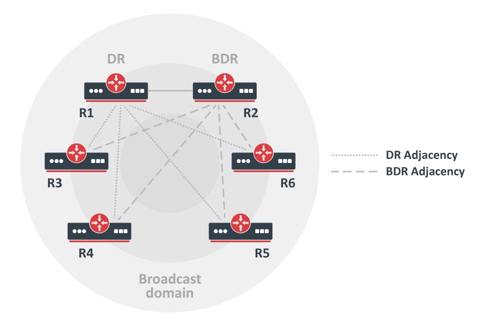
This problem is solved by electing one Designated Router and one Backup Designated Router for each broadcast subnet. All other routers are synchronizing and forming adjacencies only with those two elected routers. This approach reduces the number of adjacencies from n*(n-1)/2 to only 2n-3.
The image on the right illustrates adjacency formations on broadcast subnets. Routers R1 and R2 are Designated Routers and Backup Designated routers respectively. For example, if R3 wants to flood Link State Update (LSU) to both R1 and R2, a router sends LSU to the IP multicast address AllDRouters (224.0.0.6) and only DR and BDR listen to this multicast address. Then Designated Router sends LSU addressed to AllSPFRouters, updating the rest of the routers.
DR Election
DR and BDR routers are elected from data received in the Hello packet. The first OSPF router on a subnet is always elected as Designated Router, when a second router is added it becomes Backup Designated Router. When an existing DR or BDR fails new DR or BDR is elected to take into account configured router priority. The router with the highest priority becomes the new DR or BDR.
Being Designated Router or Backup Designated Router consumes additional resources. If Router Priority is set to 0, then the router is not participating in the election process. This is very useful if certain slower routers are not capable of being DR or BDR.
Synchronization on NBMA Subnets
Database synchronization on NBMA networks is similar to that on broadcast networks. DR and BDR are elected, databases initially are exchanged only with DR and BDR routers and flooding always goes through the DR. The only difference is that Link State Updates must be replicated and sent to each adjacent router separately.
Synchronization on PTMP Subnets
On PTMP subnets OSPF router becomes adjacent to all other routes with which it can communicate directly.
Understanding OSPF Areas
A distinctive feature of OSPF is the possibility to divide AS into multiple routing Areas which contain their own set of neighbors.
Imagine a large network with 300+ routers and multiple links between them. Whenever link flaps or some other topology change happens in the network, this change will be flooded to all OSPF devices in the network resulting in a quite heavy load on the network and even downtime since network convergence may take some time for such a large network.
A large single-area network can produce serious issues:
- Each router recalculates the database every time whenever network topology change occurs, the process takes CPU resources.
- Each router holds an entire link-state database, which shows the topology of the entire network, it takes memory resources.
- A complete copy of the routing table and a number of routing table entries may be significantly greater than the number of networks, which can take even more memory resources.
- Updating large databases requires more bandwidth.
The introduction of areas allows for better resource management since topology change inside one area is not flooded to other areas in the network. The concept of areas enables simplicity in network administration as well as routing summarization between areas significantly reducing the database size that needs to be stored on each OSPF neighbor. This means that each area has its own link-state database and corresponding shortest-path tree.
The structure of an area is invisible to other areas. This isolation of knowledge makes the protocol more scalable if multiple areas are used; routing table calculation takes fewer CPU resources and routing traffic is reduced.
However, multi-area setups create additional complexity. It is not recommended to separate areas with fewer than 50 routers. The maximum number of routers in one area is mostly dependent on the CPU power you have for routing table calculation.
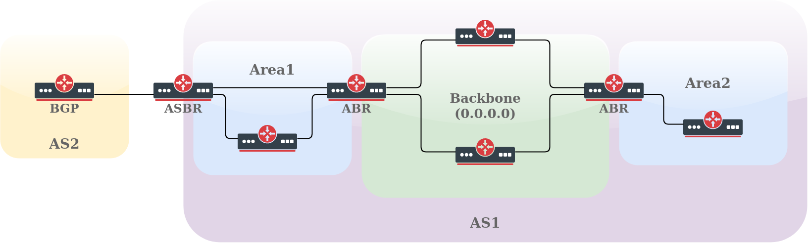
OSPF area has unique 32-bit identification (Area ID) and the area with an Area ID of 0.0.0.0 (called the Backbone area) is the main one where any other area should connect. Routers that connect to more than one area are called ABR (Area Border Routers), and their main responsibility is summarization and update suppression between connected areas. The router connecting to another routing domain is called ASBR (Autonomous System Boundary Router).
Each area has its own link-state database, consisting of router-LSAs and network-LSAs describing how all routers within that area are interconnected. Detailed knowledge of the area’s topology is hidden from all other areas; router-LSAs and network-LSAs are not flooded beyond the area’s borders. Area Border Routers (ABRs) leak addressing information from one area into another in OSPF summary-LSAs. This allows one to pick the best area border router when forwarding data to destinations from another area and is called intra-area routing.
Routing information exchange between areas is essentially a Distance Vector algorithm and to prevent algorithm convergence problems, such as counting to infinity, all areas are required to attach directly to the backbone area making a simple hub-and-spoke topology. The area-ID of the backbone area is always 0.0.0.0 and can not be changed.
RouterOS area configuration is done in the /routing/ospf/area menu. For example, a configuration of an ABR router with multiple attached areas, one Stub area, and one default area:
/routing ospf area
add name=backbone_v2 area-id=0.0.0.0 instance=v2inst
add name=stub_area area-id=1.1.1.1 instance=v2inst type=stub
add name=another_area area-id=2.2.2.2 instance=v2inst type=default
OSPF can have 5 types of areas. Each area type defines what type of LSAs the area supports:
- standard/default — OSPF packets can normally be transmitted in this area, it supports types 1,2,3,4 and 5 LSAs
- backbone — as already mentioned this is the main area where any other area connects. It is basically the same as the standard area but identified with ID 0.0.0.0
- stub — this area does not accept any external routes
- totally stubby — a variation of the stub area
- not-so-stubby (NSSA) — a variation of the stub area
LSA Types
Before we continue a detailed look at each area type, let’s get familiar with LSA types:
- type 1 — (Router LSA) Sent by routers within the Area, including the list of directly attached links. Do not cross the ABR or ASBR.
- type 2 — (Network LSA) Generated for every «transit network» within an area. A transit network has at least two directly attached OSPF routers. Ethernet is an example of a Transit Network. A Type 2 LSA lists each of the attached routers that make up the transit network and is generated by the DR.
- type 3 — (Summary LSA) The ABR sends Type 3 Summary LSAs. A Type 3 LSA advertises any networks owned by an area to the rest of the areas in the OSPF AS. By default, OSPF advertises Type 3 LSAs for every subnet defined in the originating area, which can cause flooding problems, so it´s a good idea to use a manual summarization at the ABR.
- type 4 — (ASBR-Summary LSA) It announces the ASBR address, it shows “where” the ASBR is located, announcing its address instead of its routing table.
- type 5 — (External LSA) Announces the Routes learned through the ASBR, are flooded to all areas except Stub areas. This LSA divides into two sub-types: external type 1 and external type 2.
- type 6 — (Group Membership LSA) This was defined for Multicast extensions to OSPF and is not used by RouterOS.
- type 7 — type 7 LSAs are used to tell the ABRs about these external routes imported into the NSSA area. Area Border Router then translates these LSAs to type 5 external LSAs and floods as normal to the rest of the OSPF network
- type 8 — External Attributes LSA (OSPFv2) / link-local LSA (OSPFv3)
- type 9 — Link-Local Scope Opaque (OSPFv2) / Intra Area Prefix LSA (OSPFv3). LSA of this type is not flooded beyond the local (sub)network.
- type 10 — Area Local Scope Opaque. LSA of this type is not flooded beyond the scope of its associated area.
- type 11 — Opaque LSA which is flooded throughout the AS (scope is the same as type 5). It is not flooded in stub areas and NSSAs.
If we do not have any ASBR, there are no LSA Types 4 and 5 in the network.
Standard Area
This area supports 1, 2, 3, 4, and 5 LSAs.
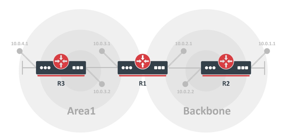
Simple multi-area network using default area. In this example, all networks from area1 are flooded to the backbone and all networks from the backbone are flooded to area1.
R1:
/ip address add address=10.0.3.1/24 interface=ether1
/ip address add address=10.0.2.1/24 interface=ether2
/routing ospf instance
add name=v2inst version=2 router-id=1.0.0.1
/routing ospf area
add name=backbone_v2 area-id=0.0.0.0 instance=v2inst
add name=area1 area-id=1.1.1.1 type=default instance=v2inst
/routing ospf interface-template
add networks=10.0.2.0/24 area=backbone_v2
add networks=10.0.3.0/24 area=area1
R2:
/ip address add address=10.0.1.1/24 interface=ether2
/ip address add address=10.0.2.2/24 interface=ether1
/routing ospf instance
add name=v2inst version=2 router-id=1.0.0.2
/routing ospf area
add name=backbone_v2 area-id=0.0.0.0
/routing ospf interface-template
add networks=10.0.2.0/24 area=backbone_v2
add networks=10.0.1.0/24 area=backbone_v2
R3:
/ip address add address=10.0.3.2/24 interface=ether2
/ip address add address=10.0.4.1/24 interface=ether1
/routing ospf instance
add name=v2inst version=2 router-id=1.0.0.3
/routing ospf area
add name=area1 area-id=1.1.1.1 type=stub instance=v2inst
/routing ospf interface-template
add networks=10.0.3.0/24 area=area1
add networks=10.0.4.0/24 area=area1
Stub Area
The main purpose of stub areas is to keep such areas from carrying external routes. Routing from these areas to the outside world is based on a default route. A stub area reduces the database size inside an area and reduces the memory requirements of routers in the area.
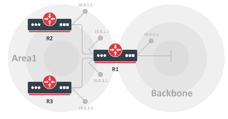
The stub area has a few restrictions, ASBR routers cannot be internal to the area, stub area cannot be used as a transit area for virtual links. The restrictions are made because the stub area is mainly configured not to carry external routes.
This area supports 1, 2, and 3 LSAs.
Let’s consider the example above. Area1 is configured as a stub area meaning that routers R2 and R3 will not receive any routing information from the backbone area except the default route.
R1:
/routing ospf instance
add name=v2inst version=2 router-id=1.0.0.1
/routing ospf area
add name=backbone_v2 area-id=0.0.0.0 instance=v2inst
add name=area1 area-id=1.1.1.1 type=stub instance=v2inst

/routing ospf interface-template
add networks=10.0.0.0/24 area=backbone_v2
add networks=10.0.1.0/24 area=area1
add networks=10.0.3.0/24 area=area1
R2:
/routing ospf instance
add name=v2inst version=2 router-id=1.0.0.2
/routing ospf area
add name=area1 area-id=1.1.1.1 type=stub instance=v2inst
/routing ospf interface-template
add networks=10.0.1.0/24 area=area1
R3:
/routing ospf instance
add name=v2inst version=2 router-id=1.0.0.3
/routing ospf area
add name=area1 area-id=1.1.1.1 type=stub instance=v2inst
/routing ospf interface-template
add networks=10.0.3.0/24 area=area1
Totally Stubby Area
Totally stubby area is an extension of the stub area. A totally stubby area blocks external routes and summarized (inter-area) routes from going into the area. Only intra-area routes are injected into the area. Totally stubby area is configured as a stub area with an additional no-summaries flag. This area supports Type 1, Type 2 LSAs, and Type 3 LSAs with default routes.
/routing ospf area
add name=totally_stubby_area area-id=1.1.1.1 instance=v2inst type=stub no-summaries
NSSA
Not-so-stubby area (NSSA) is useful when it is required to inject external routes, but injection of type 5 LSA routes is not required.
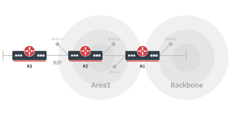
The illustration shows two areas (backbone and area1) and RIP connection to the router located in «area1». We need «area1» to be configured as a stub area, but it is also required to inject external RIP routes in the backbone. Area1 should be configured as NSSA in this case.
The configuration example does not cover RIP configuration.
R1:
/routing ospf instance
add name=v2inst version=2 router-id=1.0.0.1
/routing ospf area
add name=backbone_v2 area-id=0.0.0.0 instance=v2inst
add name=area1 area-id=1.1.1.1 type=nssa instance=v2inst
/routing ospf interface-template
add networks=10.0.0.0/24 area=backbone_v2
add networks=10.0.1.0/24 area=area1
R2:
/routing ospf instance
add name=v2inst version=2 router-id=1.0.0.2
/routing ospf area
add name=area1 area-id=1.1.1.1 type=nssa instance=v2inst
/routing ospf interface-template
add networks=10.0.1.0/24 area=area1
Virtual links cannot be used over NSSA areas.
External Routing Information and Default Route
On the edge of an OSPF routing domain, you can find routers called AS boundary routers (ASBRs) that run one of the other routing protocols. The job of those routers is to import routing information learned from other routing protocols into the OSPF routing domain. External routes can be imported at two separate levels depending on the metric type.
- type1 — OSPF metric is the sum of the internal OSPF cost and the external route cost
- type2 — OSPF metric is equal only to the external route cost.
External routes can be imported via the instance redistribute parameter. The example below will pick and redistribute all static and RIP routes:
/routing ospf instance
add name=v2inst version=2 router-id=1.2.3.4 redistribute=static,rip
Redistribution of default route is a special case where the originate-default the parameter should be used:
/routing ospf instance
set v2inst originate-default=if-installed
Since redistribution is controlled by «originate-default» and «redistribute» parameter, it introduces some corner-cases for default route filtering.
- if
redistributeis enabled, then pick all routes matching redistribute parameters - If
originate-default=never, a default route will be rejected - run selected routes through
out-select-chain(if configured) - run selected routes through
out-filter-chain(if configured) - if
originate-defaultis set toalwaysorif-installed:- OSPF creates a fake default route without attributes;
- runs this route through
out-filter-chainwhere attributes can be applied, but action is ignored (always accept);
For a complete list of redistribution values, see the reference manual.
Route Summarisation
Route summarization is a consolidation of multiple routes into one single advertisement. It is normally done at the area boundaries (Area Border Routers).
It is better to summarise in the direction of the backbone. That way the backbone receives all the aggregated routes and injects them into other areas already summarized. There are two types of summarization: inter-area and external route summarization.
Inter-area route summarization works on area boundaries (ABRs), it does not apply to external routes injected into OSPF via redistribution. By default, ABR creates a summary LSA for each route in a specific area and advertises it in adjacent areas.
Using ranges allows for creating only one summary LSA for multiple routes and sending only a single advertisement into adjacent areas, or suppressing advertisements altogether.
If a range is configured with the ‘advertise‘ parameter, a single summary LSA is advertised for each range if there are any routes under the range in the specific area. Otherwise (when ‘advertise‘ parameter disabled) no summary LSAs are created and advertised outside area boundaries at all.
Inter-area route summarization can be configured from the OSPF area range menu.
Let’s consider that we have two areas backbone and area1, area1 has several /24 routes from the 10.0.0.0/16 range and there is no need to flood the backbone area with each /24 subnet if it can be summarized. On the router connecting area1 with the backbone we can set up the area range:
/routing ospf area range
add prefix=10.0.0.0/16 area=area1 advertise=yes cost=10
For an active range (i.e. one that has at least one OSPF route from the specified area falling under it), a route with the type ‘blackhole’ is created and installed in the routing table.
External route summarization can be achieved using routing filters. Let’s consider the same example as above except that area1 has redistributed /24 routes from other protocols. To send a single summarised LSA, a blackhole route must be added and an appropriate routing filter to accept only summarised route:
/ip route add dst-address=10.0.0.0/16 blackhole
/routing ospf instance
set v2inst out-filter-chain=ospf_out
/routing filter rule
add chain=ospf_out rule="if (dst == 10.0.0.0/16) {accept} else {reject}"
Virtual Link
As it was mentioned previously all OSPF areas have to be attached to the backbone area, but sometimes the physical connection is not possible. To overcome this, areas can be attached logically by using virtual links.
There are two common scenarios when virtual links can be used:
- to glue together the fragmented backbone area
- to connect remote are without direct connection to the backbone
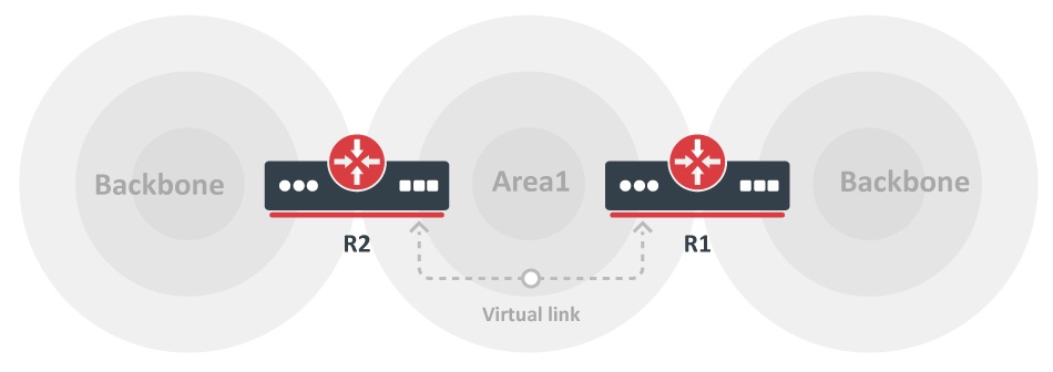
Partitioned Backbone
OSPF allows to linking of discontinuous parts of the backbone area using virtual links. This might be required when two separate OSPF networks are merged into one large network. Virtual links can be configured between separate ABRs that touch the backbone area from each side and have a common area.
The additional area could be created to become a transit area when a common area does not exist, it is illustrated in the image above.
Virtual Links are not required for non-backbone areas when they get partitioned. OSPF does not actively attempt to repair area partitions, each component simply becomes a separate area, when an area becomes partitioned. The backbone performs routing between the new areas. Some destinations are reachable via intra-area routing, the area partition requires inter-area routing.
However, to maintain full routing after the partition, an address range has not to be split across multiple components of the area partition.
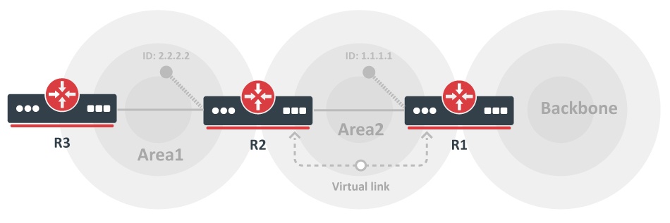
No physical connection to a backbone
The area may not have a physical connection to the backbone, a virtual link is used to provide a logical path to the backbone of the disconnected area. A link has to be established between two ABRs that have a common area with one ABR connected to the backbone.
We can see that both R1 and R2 routers are ABRs and R1 is connected to the backbone area. Area2 will be used as a transit area and R1 is the entry point into the backbone area. A virtual link has to be configured on both routers.
Virtual link configuration is added in OSPF interface templates. If we take the example setup from the «no physical connection» illustration, then the virtual link configuration would look like this:
R1:
/routing ospf interface-template
add vlink-transit-area=area2 area=backbone_v2 type=virtual-link vlink-neighbor-id=2.2.2.2
R2:
/routing ospf interface-template
add vlink-transit-area=area2 area=backbone_v2 type=virtual-link vlink-neighbor-id=1.1.1.1
Property Reference
Instance
Sub-menu: /routing/ospf/instance
| Property | Description |
|---|---|
| domain-id (Hex | Address) | MPLS-related parameter. Identifies the OSPF domain of the instance. This value is attached to OSPF routes redistributed in BGP as VPNv4 routes as BGP extended community attribute and used when BGP VPNv4 routes are redistributed back to OSPF to determine whether to generate inter-area or AS-external LSA for that route. By default Null domain-id is used, as described in RFC 4577. |
| domain-tag (integer [0..4294967295]) | if set, then used in route redistribution (as route-tag in all external LSAs generated by this router), and in route calculation (all external LSAs having this route tag are ignored). Needed for interoperability with older Cisco systems. By default not set. |
| in-filter (string) | name of the routing filter chain used for incoming prefixes |
| mpls-te-address (string) | the area used for MPLS traffic engineering. TE Opaque LSAs are generated in this area. No more than one OSPF instance can have mpls-te-area configured. |
| mpls-te-area (string) | the area used for MPLS traffic engineering. TE Opaque LSAs are generated in this area. No more than one OSPF instance can have mpls-te-area configured. |
| originate-default (always | if-installed | never; Default: never) | Specifies default route (0.0.0.0/0) distribution method. |
| out-filter-chain (name) | name of the routing filter chain used for outgoing prefixes filtering. Output operates only with «external» routes. |
| out-filter-select (name) | name of the routing filter select chain, used for output selection. Output operates only with «external» routes. |
| redistribute (bgp,connected,copy,dhcp,fantasy,modem,ospf,rip,static,vpn; ) | Enable redistribution of specific route types. |
| router-id (IP | name; Default: main) | OSPF Router ID. Can be set explicitly as an IP address, or as the name of the router-id instance. |
| version (2 | 3; Default: 2) | OSPF version this instance will be running (v2 for IPv4, v3 for IPv6). |
| vrf (name of a routing table; Default: main) | the VRF table this OSPF instance operates on |
| use-dn (yes | no) | Forces to use or ignore DN bit. Useful in some CE PE scenarios to inject intra-area routes into VRF. If a parameter is unset then the DN bit is used according to RFC. Available since v6rc12. |
Notes
OSPF protocol supports two types of metrics:
- type1 — OSPF metric is the sum of the internal OSPF cost and the external route cost
- type2 — OSPF metric is equal only to the external route cost.
Type 1 external paths are always preferred over type 2 external paths. When all paths are type 2 external paths, the paths with the smallest advertised type 2 metric are always preferred. (RFC2328)
Area
Sub-menu: /routing/ospf/area
| Property | Description |
|---|---|
| area-id (IP address; Default: 0.0.0.0) | OSPF area identifier. If the router has networks in more than one area, then an area with area-id=0.0.0.0 (the backbone) must always be present. The backbone always contains all area border routers. The backbone is responsible for distributing routing information between non-backbone areas. The backbone must be contiguous, i.e. there must be no disconnected segments. However, area border routers do not need to be physically connected to the backbone — connection to it may be simulated using a virtual link. |
| default-cost (integer; unset) | Default cost of injected LSAs into the area. If the value is not set, then stub area type-3 default LSA will not be originated. |
| instance (name; mandatory) | Name of the OSPF instance this area belongs to. |
| no-summaries () | Flag parameter, if set then the area will not flood summary LSAs in the stub area. |
| name (string) | the name of the area |
| nssa-translate (yes | no | candidate) | The parameter indicates which ABR will be used as a translator from type7 to type5 LSA. Applicable only if area type is NSSA
|
| type (default | nssa | stub; Default: default) | The area type. Read more on the area types in the OSPF case studies. |
Area Range
Sub-menu: /routing/ospf/area/range
| Property | Description |
|---|---|
| advertise (yes | no; Default: yes) | Whether to create a summary LSA and advertise it to the adjacent areas. |
| area (name; mandatory) | the OSPF area associated with this range |
| cost (integer [0..4294967295]) | the cost of the summary LSA this range will create
default — use the largest cost of all routes used (i.e. routes that fall within this range) |
| prefix (IP prefix; mandatory) | the network prefix of this range |
Interface
Sub-menu: /routing/ospf/interface
Read-only matched interface menu
Interface Templates
Sub-menu: /routing/ospf/interface-template
The interface template defines common network and interface matches and what parameters to assign to a matched interface.
Matchers
| Property | Description |
|---|---|
|
interfaces (name) |
Interfaces to match. Accepts specific interface names or the name of the interface list. |
| network (IP prefix) | the network prefix associated with the area. OSPF will be enabled on all interfaces that have at least one address falling within this range. Note that the network prefix of the address is used for this check (i.e. not the local address). For point-to-point interfaces, this means the address of the remote endpoint. |
Assigned Parameters
| Property | Description |
|---|---|
| area (name; mandatory) | The OSPF area to which the matching interface will be associated. |
| auth (simple | md5 | sha1 | sha256 | sha384 | sha512) | Specifies authentication method for OSPF protocol messages.
If the parameter is unset, then authentication is not used. |
| auth-id (integer) | The key id is used to calculate message digest (used when MD5 or SHA authentication is enabled). The value should match all OSPF routers from the same region. |
| authentication-key (string) | The authentication key to be used, should match on all the neighbors of the network segment. |
| comment(string) | |
| cost(integer [0..65535]) | Interface cost expressed as link state metric. |
| dead-interval (time; Default: 40s) | Specifies the interval after which a neighbor is declared dead. This interval is advertised in hello packets. This value must be the same for all routers on a specific network, otherwise, adjacency between them will not form |
| disabled(yes | no) | |
| hello-interval (time; Default: 10s) | The interval between HELLO packets that the router sends out this interface. The smaller this interval is, the faster topological changes will be detected, the tradeoff is more OSPF protocol traffic. This value must be the same for all the routers on a specific network, otherwise, adjacency between them will not form. |
| instance-id (integer [0..255]; Default: 0) | |
| passive () | If enabled, then do not send or receive OSPF traffic on the matching interfaces |
| prefix-list (name) | Name of the address list containing networks that should be advertised to the v3 interface. |
| priority (integer: 0..255; Default: 128) |
Router’s priority. Used to determine the designated router in a broadcast network. The router with the highest priority value takes precedence. Priority value 0 means the router is not eligible to become a designated or backup designated router at all. ROS v7 default value is 128 (defined in RFC), and the default value in ROS v6 was 1, keep this in mind when if you had strict priorities set for DR/BDR election. |
| retransmit-interval (time; Default: 5s) | Time interval the lost link state advertisement will be resent. When a router sends a link state advertisement (LSA) to its neighbor, the LSA is kept until the acknowledgment is received. If the acknowledgment was not received in time (see transmit-delay), the router will try to retransmit the LSA. |
| transmit-delay (time; Default: 1s) | Link-state transmit delay is the estimated time it takes to transmit a link-state update packet on the interface. |
| type (broadcast | nbma | ptp | ptmp | ptp-unnumbered | virtual-link; Default: broadcast) | the OSPF network type on this interface. Note that if interface configuration does not exist, the default network type is ‘point-to-point’ on PtP interfaces and ‘broadcast’ on all other interfaces.
|
| vlink-neighbor-id (IP) | Specifies the router-id of the neighbor which should be connected over the virtual link. |
| vlink-transit-area (name) | A non-backbone area the two routers have in common over which the virtual link will be established. Virtual links can not be established through stub areas. |
Lsa
Sub-menu: /routing/ospf/lsa
Read-only list of all the LSAs currently in the LSA database.
| Property | Description |
|---|---|
| age (integer) | How long ago (in seconds) the last update occurred |
| area (string) | The area this LSA belongs to. |
| body (string) | |
| checksum (string) | LSA checksum |
| dynamic (yes | no) | |
| flushing (yes | no) | |
| id (IP) | LSA record ID |
| instance (string) | The instance name this LSA belongs to. |
| link (string) | |
| link-instance-id (IP) | |
| originator (IP) | An originator of the LSA record. |
| self-originated (yes | no) | Whether LSA originated from the router itself. |
| sequence (string) | A number of times the LSA for a link has been updated. |
| type (string) | |
| wraparound (string) |
Neighbors
Sub-menu: /routing/ospf/neighbor
Read-only list of currently active OSPF neighbors.
| Property | Description |
|---|---|
| address (IP) | An IP address of the OSPF neighbor router |
| adjacency (time) | Elapsed time since adjacency was formed |
| area (string) | |
| bdr (string) | An IP address of the Backup Designated Router |
| comment (string) | |
| db-summaries (integer) | |
| dr (IP) | An IP address of the Designated Router |
| dynamic (yes | no) | |
| inactive (yes | no) | |
| instance (string) | |
| ls-requests (integer) | |
| ls-retransmits (integer) | |
| priority (integer) | Priority configured on the neighbor |
| router-id (IP) | neighbor router’s RouterID |
| state (down | attempt | init | 2-way | ExStart | Exchange | Loading | full) |
|
| state-changes (integer) | Total count of OSPF state changes since neighbor identification |
Static Neighbour configuration
Sub-menu: /routing/ospf/static-neighbor
Static configuration of the OSPF neighbors. Required for non-broadcast multi-access networks.
| Property | Description |
|---|---|
| address (IP%iface; mandatory ) | The unicast IP address and an interface, that can be used to reach the IP of the neighbor. For example, address=1.2.3.4%ether1 indicates that a neighbor with IP 1.2.3.4 is reachable on the ether1 interface. |
| area (name; mandatory ) | Name of the area the neighbor belongs to. |
| comment (string) | |
| disabled (yes | no) | |
| instance-id (integer [0..255]; Default: 0) | |
| poll-interval (time; Default: 2m) | How often to send hello messages to the neighbors which are in a «down» state (i.e. there is no traffic from them) |
-
Главная
-
Блог
-
Инфраструктура
-
OSPF-протокол: основные термины и принцип работы
OSPF представляет собой протокол маршрутизации, задачей которого является нахождение оптимального пути для передачи данных. В статье рассмотрим принцип работы протокола маршрутизации OSPF и ряд важных особенностей, понимание которых упростит работу с ним.

Чтобы понять, как работает Open Shortest Path First (так расшифровывается эта аббревиатура, которую можно перевести, как «первый кратчайший открытый путь»), нужно знать основы статической маршрутизации. Допустим, у нас есть корпоративная БД, размещенная на сервере организации. При открытии файла маршрутизатор (будем также использовать синонимы: устройство маршрутизации и роутер) получает запрос и определяет, куда направить пакет данных. Делается это с помощью таблицы маршрутизации.
Трудности начинаются, когда корпоративная инфраструктура состоит уже из нескольких сотен устройств маршрутизации. И решение в этом случае заключается в использовании динамического транспортного протокола OSPF, который автоматизирует работу маршрутизаторов, что существенно облегчает задачу системным администраторам.
Выручает OSPF и при сбоях сети. При прерывании одного из каналов связи передача пакетов данных также прекратится, поскольку статическая маршрутизация не предполагает автоматического переопределения путей. А делать это вручную при разветвленной инфраструктуре крайне трудозатратно. Если же используется OSPF, перестроение маршрутов будет происходить в автоматическом режиме.
И данные будут пересылаться до тех пор, пока есть хотя бы один доступный канал, где бы он ни был расположен внутри системы. Внутри, потому что этот протокол работает только в пределах одного домена или сетевой структуры замкнутого типа.
Терминология
Чтобы понять алгоритмы, по которым работает протокол динамической маршрутизации OSPF, нужно знать несколько несложных терминов:
- Автономная система — сетевая инфраструктура с единым управлением и настройками маршрутизации.
- Интерфейс — в данном случае является синонимом канала.
- Area — зона или система устройств маршрутизации, обменивающихся LSA и обладающих единым ID.
- LSA — пакеты данных с информацией о статусе каналов.
- Link State — состояние связи между роутерами, для обновления состояния используются LSA.
- LSU — пакет данных с содержащимися в нем LSA. Также используется термин Hello-пакет, однако различие между LSU и Hello в том, что LSU пересылают информацию о состоянии каналов связи, а Hello используются для нахождения устройств.
- Link-State DataBase — база LSA с соответствующими записями. Для ее обозначения обычно используется сокращение LSDB. Синонимичный термин: Topological DB.
- Router ID — идентификатор устройства, обычно 32-битный. Всегда является уникальным.
- Соседи — роутеры в пределах одной Area.
- Adjacency — двусторонняя связь между соседями, которые обмениваются данными о путях маршрутизации.
- Shortest Path First или SPF — так называется алгоритм, рассчитывающий оптимальные маршруты.
- Стоимость — затратность передачи данных по конкретному пути. Определяется различными факторами, а одним из важнейших является пропускная способность.
- Designated Router или DR — выделенный роутер. Управляет передачей LSA в масштабах всей сети, поэтому связан со всеми остальными устройствами.
- Backup Designated Router или BDR — резервное устройство. Этот роутер необходим в тех случаях, когда недоступен основной DR, что повышает стабильность сети. Также связан со всеми устройствами маршрутизации.
Принцип работы OSPF
Алгоритм, по которому работает OSPF, следующий:
- После включения роутеру присваивается Router ID (также можно назначить ему ID и самостоятельно).
- OSPF приступает к поиску соседних маршрутизаторов, рассылая по сети соответствующие пакеты.
- При успешном ответе между роутерами формируются каналы связи, а если ответ не был получен, маршруты автоматически перестраиваются.
- Далее происходит обмен LSA, в которых содержится нужная информация (о сетях, соседних маршрутизаторах и т. д.) для того, чтобы рассчитывать оптимальные пути передачи пакетов данных.
- Затем роутеры синхронизируют общую LSDB, в которой сохранены LSA.
- Чтобы избежать забивания каналов, задействуется Designated Router, через который пересылаются пакеты данных с информацией о состоянии всей сети и о статусе каждого роутера. DR можно назначить принудительно, а если этого не сделать, система присваивает этот статус маршрутизатору с наибольшим IP.
- Наконец, OSPF приступает к расчетам кратчайших маршрутов для сетей. Построение идет по древовидной схеме, когда от корней (роутеров) идут ветви (пути), при этом схема оптимизируется по мере необходимости.
Добавим, что работа по данному алгоритму происходит только при установленном и включенном OSPF и на роутере, и в интерфейсе. Переходим к описанию отдельных процессов маршрутизации OSPF.
Запуск
Запускаем OSPF на роутере. Идентификатор маршрутизатора будет назначен автоматически, хотя можно сделать это и вручную. Далее назначаются сети для передачи OSPF и указывается, откуда будут идти пакеты. Также назначаются сети, которые будут объявлены для других роутеров. Для этого необходимо указать номер сети, маску и номер Area. Теперь, если остальные маршрутизаторы настроены корректно, то между ними будет установлено соседство. Важно: для корректной работы интервалы передачи hello-пакетов, Area ID и интерфейсы на соседствующих роутерах должны быть идентичными.
Установка отношений
«Соседские» отношения между маршрутизаторами устанавливаются так. Допустим, у нас 4 роутера, причем четвертый будет новым, для которого нам нужно установить отношения соседства. Теперь вспоминаем терминологию. Один из роутеров у нас DR, а другой BDR.
Новый роутер рассылает hello-пакеты, а первые три, получая их, добавляют его в свои списки со статусом поиска Init. Затем соседство подтверждает и четвертый роутер. Происходит автоматическое установление 2-Way. Это тип симметричных отношений, при которых установлен обмен пакетами данных, однако обмен маршрутами пока не осуществляется.
Далее устройства пересылают друг другу служебные пакеты данных с информацией о маршрутной БД, а также запросы Link State (также называемые LSR или Link State Request). После этого происходит обмен сообщениями с детальной информацией о маршрутах и синхронизируется Link-State DataBase (Topological DB). На этом этапе устанавливаются полноценные соседствующие отношения между устройствами, в том числе с выделенным и резервным роутерами.
Распределение ролей
Как известно, в задачи DR входит управление передачей LSA в сетевом масштабе, и DR связан с остальными устройствами сети, а BDR выполняет страховочную функцию, если вдруг DR станет недоступен. Выбор выделенного и резервного маршрутизаторов может быть выполнен автоматически (на основе длины IP), либо же они могут быть назначены вручную. Также после добавления в сеть нового устройства роли DR/BDR могут быть перераспределены.
DR играет ключевую роль в обеспечении связности: он отвечает за обмен LSA-пакетами, установление соседства, синхронизацию работы устройств через обмен DBD (в этих сообщениях содержится информация о синхронизации через Topological DB). Из других особенностей отметим, что роутеры со статусом DR и BDR получают групповой адрес.
Зоны OSPF
Сетевое пространство в OSPF делится на зоны (Area), которые представляют собой логические структуры. Под термином Area понимается своеобразный сетевой кластер — определенный набор роутеров с собственной БД и топологией. При этом роутеры из других Area не располагают информацией о чужих топологиях. Зоны имеют собственные ID, которые называются Area ID. Внешне эти ID могут выглядеть как IP, однако таковыми не являются. Теперь давайте рассмотрим типы зон OSPF. Основных пять:
- Area 0. Встречаются и другие названия: магистральная, зона 0.0.0.0. Это важнейшая часть системы маршрутизации, формирующая ядро всей сети, и через нее проходит весь сетевой трафик. «Мозгом» Area 0 является Backbone Router, магистральный роутер, минимум один из интерфейсов которого относится к Area 0.
- Normal Area. Это стандартная зона, назначение которой в обновлении каналов маршрутизации, в том числе внешней.
- Transit Area. Транзитная зона, отвечающая за передачу пакетов данных между соседними областями. Area 0 также можно отнести к транзитным, но с особыми полномочиями.
- NSS Area или NSSA. Назначение этой зоны (расшифровывается как Not-So-Stubby Area) заключается в передаче пакетов данных в другие зоны, при этом она не получает информацию о путях маршрутизации извне. Поэтому для пересылки пакетов в этом месте сети используют роутер особого типа, ASBR, который как раз и способен получать такие маршруты. А для обмена данными на границах между зонами используют устройства ABR, являющиеся пограничными роутерами.
- Stub Area. Это название переводится как «тупиковая зона», и здесь невозможен прием пакетов данных, содержащих информацию о внешней маршрутизации. Однако возможен прием маршрутов из соседних зон. Также Stub Area не предназначена для размещения устройств типа ASBR, поэтому здесь задействуются пути по умолчанию. Существует и расширенный вариант под названием Totally Stub Area, где на стандартные пути заменены и остальные: не только внешние, но и между зонами.
И еще немного терминологии. Внутризональные устройства, в том числе и находящиеся в пределах зоны 0.0.0.0, называют внутренними или Internal. Особенность этих устройств в том, что они имеют зональные интерфейсы и единую Link-State DataBase. При этом каждое устройство может одновременно выступать в разных ролях, а зоны не всегда являются физическими, поскольку для их создания могут использоваться технологии виртуализации инфраструктуры.
Также существует и мультизональная структура, которая используется при значительном числе устройств маршрутизации. Мультизональная структура подходит для сегментирования сети, снижения нагрузки на аппаратную часть и для сокращения количества пересылаемых пакетов.
Типы пакетов LSA и OSPF
LSA представляет собой пакет данных с информацией о конкретном устройстве маршрутизации или отдельной сети. Из LSA формируется LSDB, причем данные пакеты имеют 11 разновидностей:
- LSA1 создаются роутерами в пределах одной зоны. В пакетах этого типа пересылаются данные об интерфейсах и особенностях внутризональных устройств.
- LSA 2 предназначены для отправки соседним внутризональным устройствам. Отправителем данных пакетов выступает выделенный роутер, а содержимое этих пакетов — информация о подключенных устройствах.
- LSA 3 содержат общие данные о путях маршрутизации соседних устройств, исключая топологическую информацию.
- LSA 4, помимо данных, передаваемых LSA 3, также содержат маршруты до локальных устройств, относящимся к соседним зонам.
- LSA 5 несут внешние данные, передаваемые в том числе по иным протоколам.
- LSA 6 — пакеты для мультиадресной маршрутизации MOSPF.
- LSA 7 работают аналогично LSA 5, однако создают ASBR при условии нахождения в NSSA.
- LSA 8 необходимы для трансляции данных BGP.
- Наконец, пакеты LSA 9, 10, 11 выполняют особые функции, расширяющие функционал протокола. С их помощью можно организовать, например, потоковое вещание.
Далее стоит отметить, что независимая передача LSA невозможна, и устройства передают эти данные только внутри пакетов OSPF. Заголовок такого пакета обычно содержит информацию о версии, типе пересылаемых данных, длине, ID устройства, зональный ID и ряд дополнительных данных. Что касается самих типов пакетов OSPF, то различают следующие разновидности:
- Hello. Используются для нахождения соседних устройств, определения их состояния и создания связей соседства с ними.
- DBD. Нужны для контроля синхронизации БД между устройствами.
- LSR. Используются для запросов фрагментов БД соседних устройств.
- LSU. Нужны для отправки данных о текущем состоянии каналов связи.
- LSAck. Предназначены для подтверждения получения каких-либо пакетов данных, пересылаемых по OSPF.
Синхронизация LSDB (Topological DB)
LSA любого типа формируют Topological DB, а каждое устройство маршрутизации имеет собственную копию этой базы данных, которую они сопоставляют с БД выделенного роутера. При этом остальные роутеры отвечают за информацию об исходящих от них связях. При изменении структуры сети (например, возникли другие связи или какие-то устройства оказались недоступны) рядовой роутер изменяет копию БД и посылает ее выделенному. За это отвечает протокол под названием Flooding. Добавим, что каждая запись в Topological DB имеет свой номер, и чем она новее, тем больше номер. Это помогает поддерживать актуальность базы данных.
Выбор оптимального маршрута
Для этого в протоколе используется специальный алгоритм. Он базируется на расчете стоимости пересылки пакетов на основе топологии. При этом стоимость определяется с учетом различных метрик (например, загруженность канала связи, его пропускная способность). Кроме того, имеется и система приоритетов. Так, при построении маршрута в первую очередь анализируются внутренние зоны, затем межзональные пути и уже потом внешние каналы передачи данных. Для расчетов используется алгоритм Дейкстры и регулярно обновляемая таблица Topological DB. При этом данная таблица каждый раз обнуляется, и маршруты выстраиваются заново с учетом новых данных. Разумеется, это довольно затратно в плане нагрузки на процессорные мощности сервера.
OSPF в Cisco и Juniper
Устройства Cisco и Juniper работают по OSPF так же, как и остальные, а различие заключается только в инструкциях. Вот сравнительные примеры проверки отношений соседства и таблицы маршрутизации на Cisco и Juniper соответственно:
Cisco:
show ip ospf neighbors
show ip route
Juniper:
root@R1> show ospf neighbor
root@R1> show route
Похоже, но реализовано чуть иначе в коде. Также, помимо базовой настройки, на оборудовании Cisco поддерживаются расширенные параметры протокола OSPF для одной области.
OSPF для IPv6
Поддержка IPv6 у OSPF имеется, однако для этого нужно использовать минимум третью версию протокола. Заметим, что вся информация выше одинаково применима ко всем версиям протокола, поэтому настройка IPv6 также не должна вызывать трудностей, поскольку выполняется аналогично процедуре настройки IPv4. После включения протокола необходимо задать ID устройства, причем потребуется сделать это вручную. Всё остальное (Area, IP, другие ID) настраивается точно так же.
Заключение
OSPF позволяет эффективно выполнять динамическую маршрутизацию локальной сетевой инфраструктуры благодаря вычислениям оптимальных маршрутов по определенным алгоритмам. Единственный недостаток протокола заключается в том, что его работа нагружает процессорные мощности и оперативную память сервера. Однако это компенсируется широкими возможностями масштабирования благодаря построению иерархии зон.